Course

March 2, 2026

Database System

Warning These notes are written primarily for my own study needs. They may not be comprehensive or suitable for everyone, so feel free to browse selectively.

Acknowledgments Part of these notes draws inspiration from the excellent Database System notes written by NoughtQ. I am also grateful to Professor Ling Chen for his teaching and guidance in the course, which helped shape the understanding reflected in these notes.

Chapter 1 Introduction

Some important conceptual knowledge ~~that is not tested in exams~~.

Chapter 2 Relational Model

2.1 Keys

superkey: A key that can uniquely identify a tuple.
candidate key: A superkey with the minimal number of attributes.
primary key: A candidate key typically underlined, which cannot or rarely changes.
foreign key: An attribute that indicates a mapping from one relation to tuples in another relation; the referenced attribute must be the primary key of the referenced relation.

tips: the differences between foreign key constraint (single arrow) and referential integrity constraint (double arrow) Foreign keys address "who you can refer to";
Referential integrity addresses "who you refer to must actually exist".
Referential integrity constraints provide a strict guarantee of data validity based on foreign key constraints, rather than a simple "containment" relationship.

2.2 Relational Algebra

Priority of Relational Operations

Projection > Selection > Cartesian Product (Multiplication) > Join, Division > Intersection > Union, Difference

Select

\sigma_p(r) = \{t\ |\ t \in r \text{ and } p(t)\}

The $p$ is called a selection predicate, which can connect multiple predicates through connectives such as AND $\wedge$ , OR $\vee$ , and NOT $\neg$ .

Project

\prod_{A_1, A_2, \dots, A_k}(r)

Obtain a relation whose tuples contain only the specified attributes.

Cartesian Product

r \times s = \{\{t, q\}\ |\ t \in r \text{ and } q \in s\}

That is cross join.

Natural Join

r \bowtie_\theta = \sigma_\theta(r \times s)

And $\theta$ is a predicate about the attributes on the pattern.

Set Operations

Union $\cup$ .
Instersect $\cap$ .
Set Difference $-$ .

Assignment

“ $\leftarrow$ “ provides a convenient method for expressing complex queries. Assignments must be used for temporary relation variables, as using them on permanent variables would modify the database.

eg.

courses\_fall\_2017 \leftarrow \Pi_{\text{course\_id}} \left( \sigma_{\text{semester} = "Fall" \land \text{year} = 2017} (\text{section}) \right)

Rename

\rho_{X(A_1, A_2, \dots, A_n)}(E)

eg.

Student(id, name) \xrightarrow{ρ_{S(sid, sname)}(Student)} S(sid, sname)

Divide

r \div s = \prod_{R - S}(r) - \prod_{R - S}((\prod_{R - S}(r) \times s) - \prod_{R - S, S}(r))

The pattern of the result of $r \div s$ is $R - S$ , where its tuples satisfy that all combinations of tuples with $S$ exist in $R$ .
eg. click here.

Aggregate Functions and Operations

_{G_1, G_2, \dots, G_n} {\Large g}_{F_1(A_1), F_2(A_2), \dots, F_n(A_n)}(E)

$E$ is an arbitrary relational algebra expression
$G_1, G_2, \ldots, G_n$ are grouping attributes (which can be empty)
$F_i$ : aggregate functions, including avg, min, max, sum, count
$A_i$ : attribute names

Outer Join

Allows us to retain tuples that do not match on the join condition

left outer join (⟕): Retains all tuples from the left relation, and attributes without matching tuples on the right are filled with null.
right outer join (⟖): Retains all tuples from the right relation, and attributes without matching tuples on the left are filled with null.
full outer join (⟗): The union of the results of the left outer join and the right outer join.

2.3 Modification of the Database

Deletion

r \leftarrow r - E

Expressing deletion using relational algebra, where $r$ is a relation and $E$ is a relational algebra query.

Insertion

r \leftarrow r \cup E

Expressing insertion using relational algebra, where $r$ is a relation and $E$ is a relational algebra expression.

eg.

account \leftarrow account \cup \{("Perryridge", A\text{-}973, 1200)\}

Insertion

r \leftarrow \prod_{F_1, F_2, \dots, F_n}(r)

Chapter 3 Introduction to SQL

3.1 Data Definition Language

char(n): Fixed-length string, with length n specified by the user.
varchar(n): Variable-length string, with maximum length n specified by the user.
int: Integer.
smallint: Smaller integer.
numeric(p, d): Fixed-point number, with total number of digits p (including the sign) and number of digits to the right of the decimal point d specified by the user.
real / double precision: Correspond to single-precision floating-point and double-precision floating-point numbers, respectively.
float(n): Floating-point number, with minimum precision n specified by the user.
date: Date, including year, month, and day, e.g., 2025-02-25.
time: Time, including hour, minute, and second, e.g., 10:47:20, 10:47:20.75.
timestamp / datetime: Timestamp, i.e., date + time, e.g., 2025-02-25 10:47:20.75.

Type conversion functions exist, such as abs(), exp(), round(), sin(), cos().

-- Basic Schema Definition

-- Define relationship
CREATE TABLE borrow (
    index int NOT NULL PRIMARY KEY,
    num NUMERIC(3, 0) DEFAULT 0,
    cno CHAR(7),
    bno CHAR(8),
    borrow_date DATETIME,
    return_date DATETIME,
    type CHAR(1),
    CONSTRAINT chk_type CHECK (type IN ('T', 'G', 'U', 'O')),
    FOREIGN KEY (cno) REFERENCES card(cno)
        ON UPDATE CASCADE,
    FOREIGN KEY (bno) REFERENCES book(bno)
        ON DELETE CASCADE
);

-- composite primary key
PRIMARY KEY (cno, bno)

-- Delete relationship
DROP TABLE borrow;

-- Clear the contents of relationship
DELETE FROM borrow;

-- Add attributes
ALTER TABLE borrow ADD attribute1, attribute2;
-- Delete attributes
ALTER TABLE borrow DROP attribute1;

3.2 Basic Structure of Selection

An example covering most of content

/*
student(id, name, age, dept, gpa)
course(id, title, credits)
takes(student_id, course_id, score)
*/

SELECT DISTINCT 
    s.gpa * 10 AS scaled_gpa, 
    'Passed' AS status
FROM student AS s, takes AS t, course AS c
WHERE s.id = t.student_id
  AND t.score NOT BETWEEN 0 AND 60
ORDER BY scaled_gpa DESC, student_name ASC
LIMIT 5 OFFSET 2;

DISTINCT Removes duplicate records;
SQL allows the use of simple arithmetic expressions on constants or attributes within query statements;
SQL strings should be enclosed in single quotes ‘;
Use AS to rename;
The ORDER BY clause sorts the query results using the keywords DESC and ASC;
The LIMIT clause is used to restrict the number of result tuples, and when combined with the OFFSET keyword, it can also specify a range of tuples to return.

Tips 1. `FROM instructor, teaches` is essentially the Cartesian product of the two;
2. Use * to select all attributes

String Operations

In SQL, column names and table names are case-insensitive, while string comparisons are case-sensitive.

SQL supports string functions.For example, removing trailing spaces from a string: TRIM(s); And SUBSTRING(name,1,5), UPPER(s.name), LOWER(name) || '@cs'(‘||’ means concatenation)

For WHERE UPPER (s. name) LIKE 'KAN%':

LIKE is used for “fuzzy matching”
‘%’ matches any string (similar to the file system’s ‘*’)
‘_’ matches any single character (similar to the file system’s ‘?’)

If you want to treat these special characters as ordinary characters, you need to use the ESCAPE keyword and add an escape character before the special characters, typically using the backslash \ as the escape character.
LIKE 'ab\%cd%' ESCAPE '\' : match all strings that start with ‘ab%cd’
LIKE 'ab\\cd%' ESCAPE '\' : match all strings that start with ‘ab\cd’

Set Operation

SQL supports the set operators $\cup,\ \cap,\ \bar{\ \ }$ from relational algebra, represented by UNION, INTERSECT, and EXCEPT respectively.

Using these operators automatically eliminates duplicate records (since sets do not allow duplicate records). If you want to retain duplicate records, you need to add the ALL keyword after the set operation keyword, i.e., UNION ALL, INTERSECT ALL, EXCEPT ALL.

Null Values

The result of any arithmetic expression containing null is null, and the result of any comparison involving null is unknown (except for IS NULL and IS NOT NULL).

SQL logical expressions have three possible outcomes: true, unknown, false.

If the evaluation result of a predicate in a WHERE clause is unknown, it is treated as false.

The comparison ... = NULL always results in null.

When duplicate records are eliminated, null values are considered identical.

Aggregate functions other than count(*) ignore records where the attribute contains null values.

Aggregate Functions

AVG (col), MIN(col), MAX(col), SUM(col), COUNT (col)

SUM and AVG require that the input values must be of numeric type, while the remaining operators can operate on non-numeric types.

-- example
SELECT AVG(s.gpa) AS avg_gpa, e.cid 
  FROM enrolled AS e, student AS s 
  WHERE e.sid = s.sid
GROUP BY e.cid
HAVING AVG(s.gpa) > 3.9;

The execution order of a query statement is: FROM -> WHERE -> GROUP -> HAVING -> SELECT -> ORDER BY

Predicates in the HAVING clause are applied after groups are formed, whereas predicates in the WHERE clause are applied before groups are formed. Therefore, aggregate functions cannot be directly used in the WHERE clause.

3.3 Nested Subqueries

SQL uses IN to check whether a tuple is a member within a certain relation.IN Can be used for enumerating sets, and can also be paired with row constructors.

SELECT DISTINCT course_id
FROM section
WHERE semester = 'Fall' AND year = 2017 AND course_id IN 
(
    SELECT course_id
    FROM section
    WHERE semester = 'Spring' AND year = 2018        
);

SELECT DISTINCT name
FROM instructor
WHERE name NOT IN ('Mozart', 'Einstein')

C <comp> SOME r is equivalent to $\exists\ t \in r (C\ \langle comp \rangle\ r)$

SELECT name
FROM instructor
WHERE salary > SOME
(
    SELECT salary
    FROM instructor
    WHERE dept_name = 'Biology'
);

C <comp> ALL r is equivalent to $\forall\ t \in r (C\ \langle comp \rangle\ r)$

SELECT dept_name
FROM instructor
GROUP BY dept_name
HAVING AVG(salary) >= ALL
(
    SELECT AVG(salary)
    FROM instructor
    GROUP BY dept_name
);

= SOME $\equiv$ IN , but != SOME $≢$ NOT IN
!= ALL $\equiv$ NOT IN , but = ALL $≢$ IN
SOME $\equiv$ ANY

When the subquery returns a non-empty result, EXISTS returns true; otherwise, it returns false.Conversely, the NOT EXISTS constructor returns the opposite result.

SELECT course_id
FROM section AS S
WHERE semester = 'Fall' AND year = 2017 AND EXISTS 
(
    SELECT *
    FROM section AS T
    WHERE semester = 'Spring' AND year = 2018 AND S.course_id = T.course_id
);

UNIQUE is used to check whether there are duplicate tuples in the result of a subquery. It returns true if there are no duplicate tuples, otherwise it returns false.

SELECT T.course_id
FROM course AS T
WHERE UNIQUE 
(
    SELECT R.course_id
    FROM section AS R
    WHERE T.course_id = R.course_id AND R.year = 2017
);

FROM also support subqueries, because all query statements return a relation.

SELECT dept_name, avg_salary
FROM 
(
    SELECT dept_name, AVG(salary)
    FROM instructor
    GROUP BY dept_name
)
AS dept_avg(dept_name, avg_salary)
WHERE avg_salary > 42000;

Common Table Expressions (CTE) are an alternative to nested subqueries in complex scenarios, providing an auxiliary statement for large queries. We can think of them as a temporary table within a query.

WITH max_budget(value) AS 
(
        SELECT MAX(budget)
        FROM department
)
SELECT budget
FROM department, max_budget
WHERE department.budget = max_budget.value;

Using RECURSIVE after WITH enables a CTE to reference itself, thereby achieving recursion in SQL queries.

WITH RECURSIVE cteSource (counter) AS 
(
    ( SELECT 1 ) 
    -- Basic items
    UNION
    ( SELECT counter + 1 FROM cteSource WHERE counter < 10 )
    -- Recursive items
)
SELECT * FROM cteSource;

Scalar subqueries return only a single value (one tuple, one attribute) (though essentially the returned result is still a relation), which can be placed in SELECT, WHERE, and HAVING clauses.

SELECT dept_name, 
(
    SELECT COUNT(*)
    FROM instructor
    WHERE department.dept_name = instructor.dept_name
) AS num_instructors
FROM department;

(SELECT COUNT(*) FROM teaches) / (SELECT COUNT(*) FROM instructor); is an integer division; to convert it into a floating-point division, you need to multiply by 1.0.

3.4 Modification of the Database

Deletion

Only a complete tuple can be deleted, not specific attributes.

DELETE FROM instructor
WHERE salary < 
(
    SELECT AVG(salary)
    FROM instructor
);

Insertion

-- Insert in order of attributes
INSERT INTO course
VALUES ('CS-437', 'Database System', 'Comp. Sci.', 4);

-- Insert attributes in a specified order
INSERT INTO course(title, course_id, credits, dept_name)
VALUES ('Database System', 'CS-437',  4, 'Comp. Sci.');

-- Insert query results
INSERT INTO instrutor
    SELECT ID, name, dept_name, 18000
    FROM student
    WHERE dept_name = 'Music' AND tot_cred > 144;

You can insert only some attributes, in which case the remaining attributes will be assigned null values.

Updates

UPDATE instructor
SET salary = salary * 1.05
WHERE salary < 
(
    SELECT AVG(salary)
    FROM instructor
);

UPDATE student
SET tot_cred = 
(
    SELECT SUM(credits)
    FROM takes, course
    WHERE student.ID = takes.ID AND
        takes.course.id = course.course_id AND
        takes.grade <> 'F' AND
        takes.graede IS NOT NULL
);

-- Supports executing different update operations conditionally within the same UPDATE statement
UPDATE instructor
SET salary = CASE
    WHEN salary <= 100000 THEN salary * 1.05
    WHEN salary BETWEEN 100000 AND 200000 THEN salary * 1.04
    ELSE salary * 1.03
END;

Chapter 4 Intermediate SQL

4.1 Join Expressions

The Natural Join

Concatenate tuples from two relations where all attributes with the same name have equal values (retaining only one of the attributes with the same name)

Order: Common attributes of the two relations - Attributes unique to the first relation - Attributes unique to the second relation

SELECT name, title
FROM (student NATURAL JOIN takes) JOIN course USING (course_id);

SELECT *
FROM student JOIN takes ON student.ID = takes.ID;
-- ON retains tuples that do not meet the conditions
-- WHERE discards tuples that do not meet the conditions

Outer Joins

LEFT OUTER JOIN: Keep only all tuples of the first relationship
RIGHT OUTER JOIN: Keep only all tuples of the second relationship
FULL OUTER JOIN: Preserve all relational tuples
INNER JOIN: Do not retain mismatched tuples

4.2 SQL and Multiset Relational Algebra

Use $\gamma$ to denote the aggregation function operation

_{dept\_name} {\Large \gamma}_{\mathbf{average}(salary)}(instructor)

SELECT A1, A2, SUM(A3)
FROM r1, r2, ..., rm
WHERE P
GROUP BY A1, A2 HAVING COUNT(A4) > 2;

Equivalent to:

\begin{aligned} & t1 \leftarrow \sigma_P(r_1 \times r_2 \times \dots \times r_m) \notag \\ & \Pi_{A_1, A_2, SumA3(\sigma_{countA4 > 2}( _{A_1, A_2} {\Large \gamma}_{sum(A_3)\ \mathbf{as}\ SumA3,\ \mathbf{count}(A_4)\ \mathbf{as}\ countA4}))}(t1) \notag \end{aligned}

semijoin $r \ltimes_{r.A = s.B} s$ : the result of $r \bowtie s$ with the attributes of $s$ removed

antijoin $\overline{\ltimes}$ ： $r - r \bowtie s$

4.3 Views

View Definition and Usages

CREATE VIEW creates a view that can be used continuously thereafter until it is manually destroyed or the program terminates.

-- template
CREATE VIEW v AS <query expression>;

-- example
CREATE VIEW faculty AS
    SELECT ID, name, dept_name
    FROM instructor;

-- You can also specify the attribute name
CREATE VIEW departments_total_salary(dept_name, total_salary) AS
    SELECT dept_name, SUM(salary)
    FROM instructor
    GROUP BY dept_name;

Materialized Views

General views only store query definitions, while materialized views also store actual data copies of the query results.

The process of keeping materialized views updated is called materialized view maintenance.

Update of a View

A view is updatable under the following conditions:

The FROM clause contains only one database relation.
The SELECT clause includes only attribute names from this relation, and no expressions, aggregate functions, or DISTINCT constraints are allowed.
Any attributes not included in the SELECT clause will be set to null, so NOT NULL or PRIMARY KEY constraints are not permitted.
The query must not include GROUP BY or HAVING clauses.

-- An example of an updatable view
CREATE VIEW history_instructors AS
SELECT *
FROM instructor
WHERE dept_name = 'History';

4.4 Transactions

A sequence of query/update statements that embodies an abstraction of the database—atomicity

COMMIT WORK: Saves changes made to the edited document
ROLLBACK WORK: Undoes all updates previously performed by SQL statements within the transaction

The database system guarantees that if a commit operation is not executed when encountering a failure, the transaction will be automatically rolled back

In many SQL implementations, by default, a single SQL statement is treated as a transaction

Disable automatic commit for individual SQL statements: SET AUTOCOMMIT OFF

Place these statements within the keywords BEGIN ATOMIC ... END, at which point these statements will be treated as a transaction

4.5 Integrity Constraints

Ensure that authorized users’ changes to the database do not compromise data consistency.

Not Null Constraint

The PRIMARY KEY constraint automatically includes this constraint, so there is no need to explicitly specify NOT NULL at this time.

Unique Constraint

UNIQUE(A_j1, A_j2, ..., A_jm)

Let the attributes $A_{j_1}, A_{j_2}, \ldots, A_{j_m}$ form a superkey

The UNIQUE constraint allows the presence of nulls (note that null values are not equal to any value, including themselves)

The Check Clause

CREATE TABLE student 
(
    id INT,
    age INT CHECK (age >= 0)
);

CREATE TABLE card 
(
    type CHAR(1),
    CONSTRAINT chk_type CHECK (type IN ('T', 'G', 'U', 'O'))
);

-- Deletion
ALTER TABLE instructor DROP CONSTRAINT minsalary;

Each tuple in the relationship must satisfy the condition of the predicate.

Without the NOT NULL constraint, null values can pass the check smoothly.

Referential Integrity

Referential integrity constraints: The specified attribute values of a certain relation (called the referencing relation) must also appear in the corresponding attributes of another relation (called the referenced relation).

CREATE TABLE employee 
(
    emp_id   INT PRIMARY KEY,
    dept_id  INT,
    mgr_id   INT,

    FOREIGN KEY (dept_id)
        REFERENCES department(dept_id)
        ON DELETE CASCADE,

    FOREIGN KEY (mgr_id)
        REFERENCES manager(mgr_id)
        ON DELETE SET NULL
);

ON DELETE CASCADE: Synchronous deletion from the referenced table to the referencing table
ON UPDATE CASCADE: Synchronous update from the referenced table to the referencing table

You can also set SET NULL or SET DEFAULT, which will be triggered when the constraint is violated

To avoid aborting transactions whenever integrity is violated, you can add the INITIALLY DEFERRED clause after the constraint declaration, specifying that the constraint should be checked only at the end of the transaction.

Complex Check Conditions and Assertions

Assertion is a predicate that expresses a condition that the database is expected to always satisfy

CREATE ASSERTION <assertion-name> CHECK <predicate>;

CREATE ASSERTION credits_earned_constraint CHECK 
(
    NOT EXISTS 
    (
        SELECT ID
        FROM student
        WHERE tot_cred <> 
        (
            SELECT COALESCE(SUM(credits), 0)
            FROM takes NATURAL JOIN course
            WHERE student.ID = takes.ID AND grade IS NOT NULL AND grade <> 'F'
        )
    )
);

for all X, P(X) == not exists X such that not P(X)

Assertion testing can incur significant overhead

4.6 SQL Data Types and Schemas

This part doesn’t seem like a key point, just skim through it to get a general impression.

4.7 Index Definition in SQL

Indexes can be established on multiple attributes.

-- tenmplate
CREATE INDEX <index-name> ON <relation-name>(<attribute-list>);

-- The key used for searching is the candidate key
CREATE UNIQUE INDEX dept_index ON instructor(dept_name);

-- Delete index
DROP INDEX <index-name>;

4.8 Authorization

Authorization of data is divided into the following categories:

Read data
Insert new data
Update data
Delete data

Granting and Revoking of Privileges

GRANT <privilege list>
ON <relation name or view name>
TO <user/role list>;

-- SELECT
GRANT SELECT ON department TO Amit, Satoshi;

-- UPDATE
GRANT UPDATE(budget) ON department TO Amit, Satoshi;

REVOKE <privilege list>
ON <relation name or view name>
TO <user/role list>;

The privilege list can include one or more of the following privileges: SELECT, INSERT, UPDATE, DELETE, ALL PRIVILEGES
PUBLIC refers to all users

Roles


-- Create a role
CREATE ROLE instructor;

-- Grant privileges to roles
GRANT SELECT ON takes TO instructor;

-- Grant a certain role to a user or other role
CREATE ROLE dean;
GRANT instructor TO dean;
GRANT dean TO Satoshi;

-- Allows user Mariano to create relations that reference 
-- the key dept_name of the department relation as a foreign key
GRANT REFERENCES(dept_name) ON department TO Mariano;

-- The privilege to grant privileges to other users
GRANT SELECT ON department TO Amit WITH GRANT OPTION;

-- cascade revocation: After revoking a user's privileges, the privileges granted by that user to other users will also be revoked.
-- Prevent cascade revocation:
REVOKE SELECT ON department FROM Amit, Satoshi RESTRICT;
-- Privileges granted can also be revoked using the REVOKE statement
REVOKE GRANT OPTION FOR SELECT ON department FROM Amit;

Users who are not granted update privileges and create views do not have update privileges on those views, and so on.

Chapter 5 Advanced SQL

5.1 Accessing SQL from Programming Languages

~~The only aspect of this section that is beneficial for grades is the JDBC syntax, and it is not included as an exam topic.~~

The methods for using SQL in general-purpose programming languages include:

Dynamic SQL: The program establishes a connection with the database server through a specific set of functions or methods. Dynamic SQL then allows the program to construct SQL queries as strings at runtime, submit the queries, and store the retrieved results in program variables.
- JDBC: An API for connecting to databases in Java.
- ODBC: An API for connecting to databases in languages such as C, C++, and C#.
Embedded SQL: A preprocessor identifies SQL statements at compile time and translates requests expressed in SQL into function call statements.

JDBC

public static void JDBCexample(String userid, String passwd) 
{
    try 
    (
        Connection conn = DriverManager.getConnection
        (
            "jdbc:oracle:thin:@db.yale:1521:univdb",
            userid,
            passwd
        );
        Statement stmt = conn.createStatement();
    )
    {
        try 
        {
            stmt.executeUpdate
            (
                "INSERT INTO instructor VALUES('77987', 'Kim', 'Physics', 98000)"
            );
        } 
        catch (SQLException sqle) 
        {
            System.out.println("Could not insert tuple. " + sqle);
        }
        ResultSet rset = stmt.executeQuery
        (
            "SELECT dept_name, AVG(salary) " + 
            "FROM instructor " +
            "GROUP BY dept_name"
        );
        while (rset.next()) 
        {
            System.out.println(rset.getString("dept_name") + " " + rset.getFloat(2));
        }

    } 
    catch (Exception sqle) 
    {
        System.out.println("Exception: " + sqle);
    }
}

Database Connection

Connection conn = DriverManager.getConnection
(
    "jdbc:oracle:thin:@db.yale:1521:univdb",
    userid,
    passwd
);

// @db.yale：Database server hostname
// :1521：Database port number
// :univdb：Database name or instance name

The first step is to establish a connection to the database.

The following parameters are accepted:

Database server information, including URL/hostname, protocol, port number, and database name.
Database username.
Password.

This method returns a Connection object.

JDBC supports multiple protocols, such as jdbc:oracle:thin for Oracle and jdbc:mysql for MySQL, among others.

Shipping SQL Statements to the Database System

Statement stmt = conn.createStatement();

Statement is an object that allows Java programs to invoke and transmit SQL statements to the database.

To execute a statement, you need to call the executeQuery() or executeUpdate() methods, which correspond to the execution of query statements and non-query statements (such as updates, inserts, deletions, creations, etc.), respectively. The latter returns a value indicating the number of tuples inserted/updated/deleted (or 0 for creation statements).

Exceptions and Resource Management

Executing any SQL statement may throw an exception, so remember to use the try {...} catch {...} block to catch exceptions when programming.

Exceptions can be categorized into SQLException (exceptions related to SQL) and Exception (exceptions related to Java).

Regarding resource management, a reliable practice is to use the try-with-resources construct, which involves adding parentheses between the try keyword and the statement block, containing resources such as connections and statement objects. This ensures that these resources are automatically closed when exiting the try block.

Retrieving the Result of Query

After using the executeQuery() method to execute a query, the retrieved tuple is placed in a ResultSet object.

This object calls the next() method to fetch the next tuple (if any), returning a boolean value indicating whether the tuple was successfully retrieved.

Methods that accept a single parameter:

getString(): Can retrieve any SQL basic data type.
getFloat(): Limited to retrieving floating-point numbers.

Prepared Statements

First, create a prepared statement where the values that appear in the statement are replaced with ? (placeholders), and then insert the specific values into the corresponding positions.

This type of method takes two parameters: the first parameter indicates which ? is being set (starting from 1), and the second parameter is the specific value.

PreparedStatement pStmt = conn.prepareStatement
    ("INSERT INTO instructor VALUES(?, ?, ?, ?)");
pStmt.setString(1, "88877");
pStmt.setString(2, "Perry");
pStmt.setString(3, "Finance");
pStmt.setInt(4, 125000);
pStmt.executeUpdate();
pStmt.setString(1, "88878");
pStmt.executeUpdate();

// Two insertion statements were executed here
// with the second insertion statement expressed in SQL syntax as:
INSERT INTO instructor VALUES("88878", "Perry", "Finance", 125000);

Callable Statements

CallableStatement interface is used to call SQL procedures or functions

CallableStatement cStmt1 = conn.prepareCall("{? = call some_function(?)}");
CallableStatement cStmt2 = conn.prepareCall("{call some_procedure(?, ?)}");

// -----------
// For example
// -----------
FUNCTION add_one(x INT) RETURNS INT
...
CallableStatement cStmt = conn.prepareCall("{? = call add_one(?)}");

// Registered return value type
cStmt.registerOutParameter(1, Types.INTEGER);

// Set input parameters
cStmt.setInt(2, 5);

// Execute
cStmt.execute();

// Get return value
int result = cStmt.getInt(1);

Metadata Features

ResultSet interface’s getMetaData(): Returns a ResultSetMetaData class object containing the metadata of the result set.

The getColumnCount() method returns the arity (i.e., the number of columns)
getColumnName() and getColumnTypeName() retrieve the column name and data type name, respectively. Both accept a single integer parameter representing the column position (starting from 1)

ResultSetMetaData rsmd = rs.getMetaData();
for (int i = 1; i <= rsmd.getColumnCount(); i++) 
{
    System.out.println(rsmd.getColumnName(i));
    System.out.println(rsmd.getColumnTypeName(i));
}

Connection interface’s getMetaData(): Returns a DatabaseMetaData class object, providing a way to access database metadata.

The getColumns() accepts four parameters: directory name, database name, table name, column name

DatabaseMetaData dbmd = conn.getMetaData();
ResultSet rs = dbmd.getColumns(null, "univdb", "department", "%");

while (rs.next()) 
{
    System.out.println(rs.getString("COLUMN_NAME"), rs.getString("TYPE_NAME"));
}

directory name: null indicates that this value is ignored
column name: Here % means to retrieve all columns

Other uses of DatabaseMetaData

getTables(): Lists all tables in the database. The first three parameters are consistent with getColumns(), and the last parameter is used to restrict tables that meet the conditions. If set to null, it returns all tables (including internal system tables).

getPrimaryKeys(): Retrieves primary keys.

getCrossReference(): Retrieves foreign key references.

Other Features

Updatable result sets: Update operations will synchronously update their corresponding relationships.

Regarding Large Objects (Blob, Clob)

Read: The ResultSet object provides getBlob() and getClob() methods, which return objects of type Blob and Clob, respectively. The principle is to store a locator (essentially a pointer), and the content of the large object can be retrieved using the getBytes() and getSubString() methods.
Write: The PreparedStatement class allows applications to use the setBlob() and setClob() methods for transmission.

Database Access from Python / ODBC / Embedded SQL

~~It’s not important for the grades, the link is attached below.~~

5.2 Functions and Procedures

Declaration and Invocation

-- ------------------------
--   function declaration
-- ------------------------

CREATE FUNCTION dept_count(dept_name VARCHAR(20)) 
    RETURNS INTEGER
    BEGIN
    DECLARE d_count INTEGER;
        SELECT COUNT(*) INTO d_count
        FROM instructor
        WHERE instructor.dept_name = dept_name;
    RETURN d_count;
    END

--- function invocation
SELECT dept_name, budget
FROM department
WHERE dept_count(dept_name) > 12;

-- ------------------------
--  return table functions
-- ------------------------

-- function declaration
CREATE FUNCTION instructor_of(dept_name VARCHAR(20))
    RETURNS TABLE
    (
        ID VARCHAR(5),
        name VARCHAR(20),
        dept_name VARCHAR(20),
        salary NUMERIC(8, 2)
    )
    RETURN TABLE
    (
        SELECT ID, name, dept_name, salary
        FROM instructor
        WHERE instructor.dept_name = instructor_of.dept_name
    );

-- function invocation
SELECT *
FROM TABLE(instructor_of('Finance'));

-- ------------------------
--  procedure declaration
-- ------------------------

CREATE PROCEDURE dept_count_proc
(
    IN dept_name VARCHAR(20),
    OUT d_count INTEGER
)
    BEGIN
        SELECT COUNT(*) INTO d_count
        FROM instructor
        WHERE instructor.dept_name = dept_count_proc.dept_name
    END

-- procedure invocation
DECLARE d_count INTEGER;
CALL dept_count_proc('Physics', d_count); -- Call process

Language Constructs

Persistent Storage Module (PSM): Similar to building blocks in other programming languages

Variable declaration and assignment are represented by DECLARE and SET statements, respectively

DECLARE count_students INT;
SET count_students = 100;

Compound statement: A block of statements composed of multiple SQL statements
- Enclosed between the BEGIN and END keywords
- Local variables can be declared within the compound statement
- A compound statement enclosed between the BEGIN ATOMIC and END keywords is treated as a single transaction

BEGIN
    DECLARE temp INT;
    SET temp = 10;
    SELECT temp;
END;

temp is only valid within this BEGIN...END block and cannot be accessed externally (similar to internal variables of a function)

Cycle

-- 1. WHILE statements
WHILE boolean expression DO
    sequence of statements;
END WHILE

-- 2. REPEAT statements
REPEAT
    sequence of statements;
UNTIL boolean expression
END REPEAT

-- 3. FOR statements
DECLARE n INTEGER DEFAULT 0;
FOR r AS       -- fetch one row at a time
    SELECT budget FROM department
    WHERE dept_name = 'Music'
DO 
    SET n = n - r.budget
END FOR

Using LEAVE and ITERATE inside a loop body is similar to the continue and break statements in programming languages.

Conditional branch

IF boolean expression
    THEN statement or compound statement
ELSE boolean expression
    THEN statement or compound statement
ELSE statement or compound statement
END IF

Exception Conditions & Handlers

DECLARE out_of_classroom_seats CONDITION
DECLARE EXIT HANDLER FOR out_of_classroom_seats
BEGIN
    sequence of statements
END

External Language Routines

-- An Example
CREATE PROCEDURE dept_count_proc
(
    IN dept_name VARCHAR(20),
    OUT count INTEGER
) 
LANGUAGE C
EXTERNAL NAME '/usr/avi/bin/dept_count_proc';

CREATE FUNCTION dept_count
(
    dept_name VARCHAR(20)
)
RETURN INTEGER
LANGUAGE C
EXTERNAL NAME '/usr/avi/bin/dept_count';

How to Handle Null Values

Set the value of the SQLSTATE class in functions/procedures to store failure/success status
Pass pointers instead of directly passing values
Add an extra line PARAMETER STYLE GENERAL in the function/procedure declaration to indicate that the function/procedure ignores null values

5.3 Triggers

To define a trigger, the following are required:

Specify the event that triggers the check
Specify the condition that must be met for the trigger to execute
Specify the actions to be performed by the trigger

-- trigger for insertion
CREATE TRIGGER timeslot_check1 AFTER INSERT ON section
REFERENCING NEW ROW AS nrow
FOR EACH ROW
WHEN 
(
    nrow.time_slot_id NOT IN 
    (
        SELECT time_slot_id
        FROM time_slot
    )
)
BEGIN
    ROLLBACK
END;

-- trigger for deletion
CREATE TRIGGER timeslot_check2 AFTER DELETE ON timeslot
REFERENCING OLD ROW AS orow
FOR EACH ROW
WHEN 
(
    orow.time_slot_id NOT IN 
    (
        SELECT time_slot_id
        FROM time_slot
    ) 
    AND orow.time_slot_id IN 
    (
        SELECT time_slot_id
        FROM section
    )
)
BEGIN
    ROLLBACK
END;

-- trigger before update
CREATE TRIGGER setnull BEFORE UPDATE OF takes
REFERENCING NEW ROW AS nrow
FOR EACH ROW
WHEN (nrow.grade = '')
    SET nrow.grade = NULL;
END;

-- trigger after update
CREATE TRIGGER credits_earned AFTER UPDATE OF takes ON grade
REFERENCING NEW ROW AS nrow 
-- Updated or newly inserted row records
REFERENCING OLD ROW AS orow 
-- Old row records that have been updated or deleted
FOR EACH ROW
WHEN nrow.grade <> 'F' AND nrow.grade IS NOT NULL
    AND (orow.grade = 'F' OR orow.grade IS NULL)
BEGIN ATOMIC
    UPDATE student
    SET tot_cred = tot_cred + 
    (
        SELECT credits
        FROM course
        WHERE course.course_id = nrow.course_id
    )
    WHERE student.id = nrow.id;
END;

Apply the trigger to all rows that satisfy the SQL at once

Change FOR EACH ROW to FOR EACH STATEMENT
And use REFERENCING OLD TABLE AS and REFERENCING NEW TABLE AS to create transition tables

Disable trigger: ALTER TRIGGER trigger_name DISABLE
Delete trigger: DROP TRIGGER trigger_name

Chapter 6 Database Design Using the E-R Model

6.1 Overview of the Design Process

Use the entity-relationship model as a data model to convert requirements into the conceptual schema of a database.
Specification of functional requirements: includes the operations (or transactions) that users need to perform on the data.
Convert the abstract data model into the concrete implementation of the database, divided into:
- Physical design: specifies the physical functions of the database, including file organization forms, index structures, etc.
- Logical design: maps the high-level conceptual schema to the concrete implementation of the data model.

Design Pitfalls: redundancy & incompleteness

6.2 The Entity-Relationship Model

It includes the following three basic concepts: entity set, relationship set, and attribute

Entity Sets

In an E-R diagram, we use a rectangle to represent an entity set, which is divided into two parts: the upper half contains the name of the entity set, while the lower half includes the names of all attributes.

Relationship Sets

degree: The number of entity sets involved in a relationship set
relationship instance: An association representing multiple named entities

In an E-R diagram, we use a diamond to represent a relationship set.

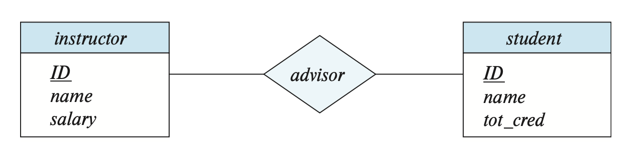
The term “participation” can be used to denote the association between entity sets, meaning that $E_1, E_2, \dots, E_n$ participate in the relationship set $R$ .

Recursive relationship set: When the same entity plays different roles in the same relationship, the role names of the entity need to be explicitly indicated.

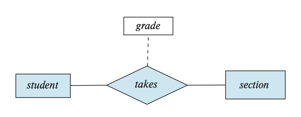
A relationship may also have a set of attributes, known as descriptive attributes, which are represented in an E-R diagram by a separate rectangle connected to the diamond with a dashed line, as shown in the figure below.

6.3 Complex Attributes

Simple Attributes and Composite Attributes

Simple attribute: An attribute that cannot be further subdivided.
Composite attribute: An attribute that can be further divided into multiple subparts (attributes).

Single-valued attributes and multivalued attributes

Single-valued attribute: An attribute with only one value
Multi-valued attribute: An attribute that can contain zero or more values

Derived attribute: This attribute derives its value from other attributes or entities.

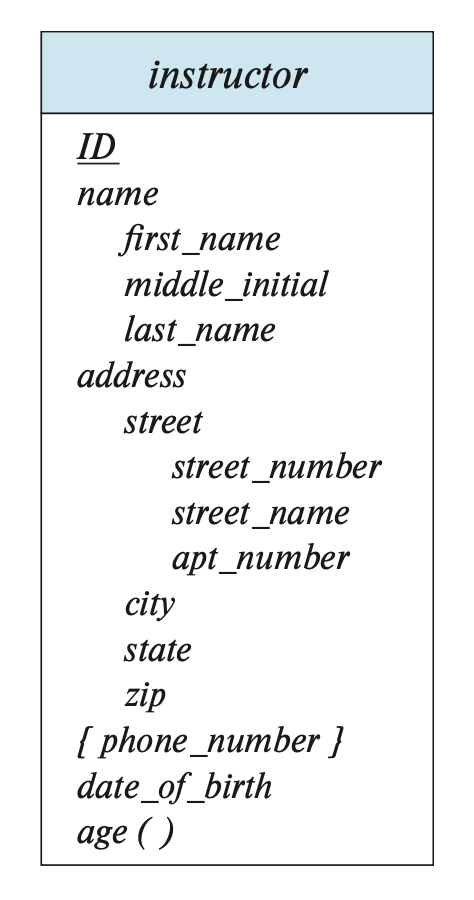
Composite attributes: Corresponding component attributes are placed directly below the composite attribute, with an indentation at the beginning.
Multi-valued attributes: Enclosed in curly braces.
Derived attributes: End with parentheses.

Different Meanings of Null Values for Attributes: not applicable / missing / unknown

6.4 Mapping Cardinalities

The number of other entities that an entity can associate with through a relationship set.

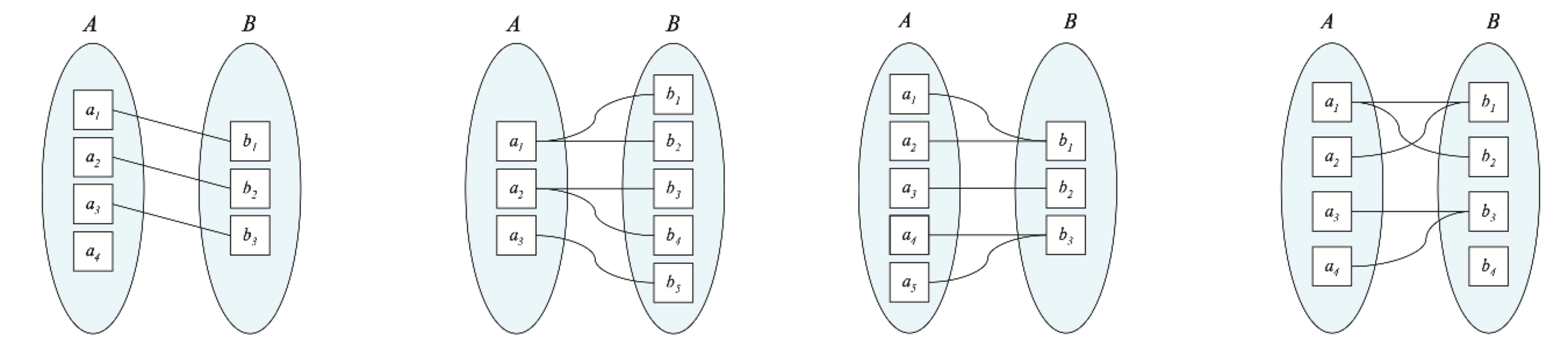
One-to-one: An entity in A is associated with at most one entity in B, and an entity in B is associated with at most one entity in A.
One-to-many: An entity in A can be associated with any number of entities in B, but an entity in B is associated with at most one entity in A.
Many-to-one: An entity in A is associated with at most one entity in B, but an entity in B can be associated with any number of entities in A.
Many-to-many: An entity in A can be associated with any number of entities in B, and an entity in B can be associated with any number of entities in A.

In an E-R diagram, we use lines with arrows (->) or without arrows (——) to represent cardinality constraints in relationships, as shown below:

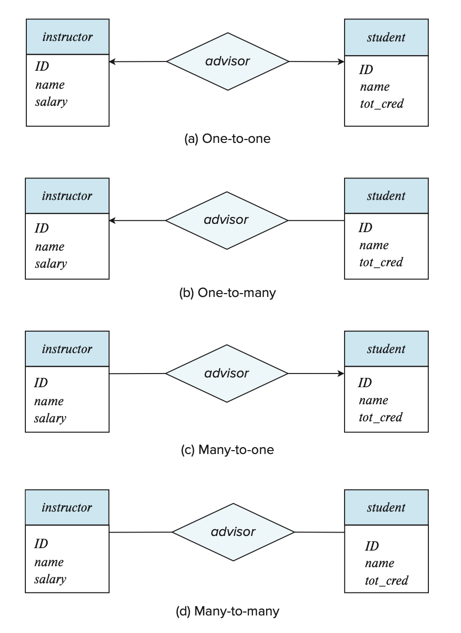
The arrow line points to the entity set of “one”.

All entities in entity set E participate in at least one relationship in relationship set R, then E is said to totally participate in R.
In an E-R diagram, we use double lines to indicate total participation.

If there exist some entities that do not participate in any relationship in R, then E is said to partially participate in R.

In an E-R diagram, we can also indicate more complex constraints—by labeling the lines with l..h, where l and h represent the minimum and maximum cardinalities, respectively. If h = *, it indicates that there is no maximum limit; if l = h = 1, it represents a one-to-one relationship.

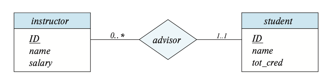
	单线	双线
箭头	0..1	1..1
无箭头	0..*	1..*

6.5 Primary Key

Entity Sets

In fact, the concepts related to keys in relational schemas (including superkeys, candidate keys, and primary keys) can be directly applied to entity sets.

Relationship Sets

Let $R$ be a relationship set involving entity sets $E_1, E_2, \dots, E_n$ , where $primary-key(E_i)$ denotes the primary key of $E_i$ , and assume that all attribute names of the primary keys are unique, and there are attributes $a_1, \dots, a_m$ associated with $R$ . The composition of the primary key of $R$ is:

primary-key(E_1) \cup primary-key(E_2) \cup \dots \cup primary-key(E_n) \cup \{a_1, a_2, \dots, a_m\}

Among them

primary-key(E_1) \cup primary-key(E_2) \cup \dots \cup primary-key(E_n)

is sufficient to form a superkey of the relationship set

If the attribute names of the primary key are not unique, it is necessary to rename these duplicate-named attributes. The naming rule is: entity_set_name.attribute_name or role_name.attribute_name

The choice of primary key also depends on the mapping cardinality:

Many-to-many: The superkey mentioned above serves as the primary key.
One-to-many, many-to-one: The primary key of the entity set on the “many” side is used as the primary key for the entire relationship set.
One-to-one: The primary key of either entity set can serve as the primary key for the relationship set.

For non-binary relationships, if no cardinality constraints are provided, the aforementioned superkey is the only candidate key, i.e., the primary key. However, if there are cardinality constraints, the situation becomes quite complex.

We stipulate: In an E-R diagram, each relationship set is allowed to have only one line with an arrow.

Weak Entity Sets

weak entity set: the existence depends on this connection set as well as another entity set (indentifying entity set).

We will use the primary key of the identifying entity set, along with some additional attributes, to identify a unique weak entity. These attributes are collectively referred to as discriminator attributes.
An identifying relationship is a many-to-one relationship from the weak entity set to the identifying entity set, and the weak entity set fully participates in this relationship.

In an E-R diagram, we use a double-layered rectangle to represent a weak entity set, with its discriminant attributes identified by a dashed underline; a double-layered diamond is used to represent an identifying relationship (connecting the weak entity set and the identifying entity set).

The primary key of a weak entity set includes the union of the primary keys of these identifying entity sets, plus the weak entity set’s own discriminant attributes.

6.6 Removing Redundant Attributes in Entity Sets

Suppose there are two entity sets $E_1, E_2$ , which are connected through a certain attribute $a$ . Both entity sets have this attribute $a$ , but in $E_1$ , this attribute is a primary key. To avoid redundancy, we need to remove the attribute $a$ from $E_2$ .

It can be understood that $R$ is a table between $E_1, E_2$ that can store mapping information.

6.7 Reducing E-R Diagrams to Relational Schemas

Strong Entity Sets

If the strong entity set has non-simple attributes:

Composite attributes - We need to create a separate attribute for each component attribute, but there is no need to create an attribute for the composite attribute itself.
Multivalued attributes - It is necessary to create a new relational schema for these attributes.
- Assuming there is a multivalued attribute M, we create a relational schema R for it, which has an attribute A corresponding to M, as well as the primary key from the entity set or relationship set where M is located.
- Create a foreign key constraint for R. The attributes in R generated from the primary key of the entity set must reference the relation generated from the entity set.

In plain language, it means creating a separate table, but using a primary key to maintain a connection with the main table.

Derived attributes - These are not explicitly represented in the relational data model but are instead represented through procedures, functions, or methods in other data models.

Weak Entity Sets

Suppose there is a weak entity set A with attributes $a_1, a_2, \dots, a_m$ , and a strong entity set B with attributes $b_1, b_2, \dots, b_n$ , on which A depends. We still refer to the relational schema corresponding to A as A, and the attributes of this relational schema are:

\{a_1, a_2, \dots, a_m\} \cup \{b_1, b_2, \dots, b_n\}

The primary key of this relationship schema is the combination of the primary key of the strong entity set and the discriminator attribute of the weak entity set.
Additionally, the foreign key constraints of this relationship schema must also be considered.

Relationship Sets

Let R be a relationship set, $a_1, a_2, \dots, a_m$ be the union of the primary keys of the entity sets participating in this relationship set, and $b_1, b_2, \dots, b_n$ be the descriptive attributes of R (if any). We still refer to the relational schema corresponding to R as R, and the attributes of this relational schema are:

\{a_1, a_2, \dots, a_m\} \cup \{b_1, b_2, \dots, b_n\}

The primary key of this relationship schema is the primary key of the relationship set.
- Additionally, the foreign key constraints of this relationship schema must also be considered.

Redundancy of Schemas
Those relationship sets that connect weak entity sets to their corresponding strong entity sets provide redundant information in their corresponding relational schemas, and therefore do not need to be represented.

Combination of Schemas

From the many-to-one relationship set AB between entity set A and entity set B, using the conversion method described above, we obtain three schemas: A, B, and AB. Assuming that A fully participates in the relationship, we can combine the schemas corresponding to A and AB into a single schema, which includes the union of the attributes from both schemas. The primary key of this combined schema is the primary key of the entity set that was merged.

For one-to-one relationships, the relationship schema of the relationship set can be combined with the relationship schema of either entity set.

Even if some entity sets are partially participating, we can still combine schemas, using null values to fill in the non-participating parts (i.e., missing tuples).

6.8 Extended E-R Features

Specialization

A top-down process for specifying subgroups from an entity set
In an E-R diagram, we use a hollow arrow pointing from the specialized entity to another entity to represent the specialization relationship.

Specialization is divided into two categories:

Overlapping specialization: An entity can belong to multiple specialized entity sets, represented by separate arrows in an E-R diagram.
Disjoint specialization: An entity can belong to at most one specialized entity set, represented by a merged arrow in an E-R diagram.

Generalization

Generalization is the inverse process of specialization

A bottom-up process in which multiple entity sets are merged into a higher-level entity set based on common characteristics.

Inheritance

In a hierarchy, inheritance can be categorized as:

Single inheritance: Each entity set in the hierarchy serves as a lower-level entity set in only one ISA relationship.
Multiple inheritance: Each entity set in the hierarchy can serve as a lower-level entity set in multiple ISA relationships, forming a structure known as a lattice.

Constraints on Specializations

Disjointness constraints: These refer to the mutually exclusive specialization and overlapping specialization mentioned earlier.

Completeness constraints: In specialization/generalization, whether entities in the higher-level entity set must belong to at least one entity in the lower-level entity set, including:

Total specialization/generalization: Every higher-level entity must belong to a lower-level entity set.
Partial specialization/generalization: Some higher-level entities may not belong to any lower-level entity set. This is the default behavior.

Aggregation

Treating a connection as an entity allows for establishing connections on this “connection” itself, while avoiding more complex expressions.

Reduction to Relation Schemas

Generalization：

Create tables for each layer. Store both “parent class” and “child class” separately, with child classes “pointing” to parent classes via primary keys.
When they are mutually disjoint and total, it is possible not to create a parent table.

Aggregation：Directly convert the aggregated relationship sets and entity sets (a larger entity set) using the previously introduced method.

Common Mistakes in E-R Diagrams
The primary key of one entity set serves as an attribute of another entity set, rather than using a relationship to associate the two. This not only creates an undesirable implicit relationship but also leads to redundant information.

Chapter 7 Relational Database Design

7.1 Introduction

Decomposition

Decompose a schema containing redundant information into several smaller schemas without redundancy.

Lossy decomposition: The resulting schemas from decomposition are non-redundant, but the schema obtained by naturally joining them back together contains more redundancy.
Lossless decomposition: The opposite.

Normalization Theory

Methodology for avoiding duplicate information issues when designing relational databases.

7.2 Functional Dependencies

Keys and Functional Dependencies

functional dependencies: a set of constraints used to identify uniquely specific attribute values in a relation

For a relation schema $r(R)$ and its attributes $\alpha, \beta \subseteq R$

For an instance of $r(R)$ , if for all its tuple pairs $t_1, t_2$ , when $t_1[\alpha] = t_2[\alpha]$ , it holds that $t_1[\beta] = t_2[\beta]$ , then the instance is said to satisfy the functional dependency $\alpha \rightarrow \beta$
If all instances of $r(R)$ satisfy the functional dependency $\alpha \rightarrow \beta$ , then the dependency is said to hold on $r(R)$

Therefore, there may be instances that satisfy some functional dependencies that do not hold over the entire relation schema

Redefine superkey using the concept of functional dependency: $K \rightarrow R$ holds on $r(R)$

For a functional dependency $\alpha \rightarrow \beta$ , if $\beta \subseteq \alpha$ , then this functional dependency is trivial.

Closure: the complete set of all functional dependencies derived from the functional dependency set F.

Lossless Decomposition and Functional Dependencies

Defining lossless decomposition using functional dependencies:

Now we define lossless decomposition using functional dependencies: when $R_1 \cap R_2 \rightarrow R_1 / R_2$ is satisfied, $R_1,R_2$ form a lossless decomposition of $R$ .

In other words, if $R_1 \cap R_2$ is a superkey for $R_1 / R_2$ , then this decomposition is lossless.
Intuitively, as long as the field used for joining is the primary key (or superkey) of one of the tables, no information will be lost.

If the relational schema $r(R)$ is decomposed into $r_1(R_1), r_2(R_2)$ , where $R_1 \cap R_2 \rightarrow R_1$ , the following SQL constraints must be added to the resulting schemas:

$R_1 \cap R_2$ is the primary key of $r_1$
$R_1 \cap R_2$ is a foreign key in $r_2$ referencing $r_1$ , ensuring that every tuple in $r_2$ can match a tuple in $r_1$

If $r_1, r_2$ are further decomposed, the key join fields must not be split apart.

7.3 Normal Forms

Boyce-Codd Normal Form

Regarding the relation $R$ with the set of functional dependencies $F$ , for all functional dependencies $\alpha \rightarrow \beta$ in $F^+$ , where $\alpha \subseteq R, \beta \subseteq R$ , $R$ is said to be in BCNF if at least one of the following conditions holds:

$\alpha \rightarrow \beta$ is a trivial functional dependency
$\alpha$ is a superkey for schema $R$

In simple terms, as long as a functional dependency is “non-trivial,” its left-hand side must be a superkey.

For schemas that do not comply with BCNF, we need to decompose them into:

$(\alpha \cup \beta)$ , placing the "determining factor" and the "determined attribute" together
$(R - (\beta - \alpha))$ , remove the redundancy from the original relationship

Continue decomposing until all results adhere to BCNF.

Dependency Preservation: Suppose a relation $R$ has a set of functional dependencies $F$ . After decomposition, we obtain subrelations $R_1, R_2, \dots R_n$ with corresponding sets of functional dependencies $F_1, F_2, \dots F_n$ . If $(F_1 \cup F_2 \cup \dots \cup F_n)^+ = F^+$ , then the decomposition is said to be dependency preserving.

Decompositions that follow the BCNF schema are not necessarily dependency preserving.

Third Normal Form

Regarding a relation $R$ with a set of functional dependencies $F$ , for all functional dependencies $\alpha \rightarrow \beta$ in $F^+$ , where $\alpha \subseteq R, \beta \subseteq R$ , $R$ is said to be in the third normal form (3NF) if at least one of the following conditions is satisfied:

$\alpha \rightarrow \beta$ is a trivial functional dependency
$\alpha$ is a superkey for schema $R$
Each attribute $A$ in $\beta - \alpha$ is a member of a (possibly different) candidate key of $R$

The third condition allows non-trivial functional dependencies whose left-hand side is not a superkey to still conform to this normal form. This more relaxed condition enables 3NF to ensure that the original dependencies are preserved during schema decomposition.

The drawback is that it may introduce null values, indicating the presence of information redundancy.

If BCNF and dependency preservation cannot be satisfied simultaneously, prioritize BCNF.

More Normal Forms

4NF: Will be discussed below
5NF: Based on a generalized multi-valued dependency—join dependencies, also known as project-join normal form (PJNF). The drawback of this normal form is not only that it is difficult to reason about, but also that its inference rules lack soundness and completeness.
2NF: Its issues can be resolved by 3NF.
1NF: Will be discussed below.

Atomic Domains and First Normal Form

First Normal Form: In a relational schema $R$ , all attribute domains must be atomic (i.e., indivisible into smaller units).

Issues arising from non-atomicity include: complex storage, redundant data, and complicated queries.

For composite attributes: Use their component attributes directly.
For multivalued attributes: Multiple fields / a separate table / a single field.

7.4 Functional-Dependency Theory

Closure of Functional Dependencies

logically implied: For a given relation schema $r(R)$ , if every instance that satisfies the set of functional dependencies $F$ also satisfies the functional dependency $f$ , then it is said that $f$ on $R$ is logically implied by $F$ .

Armstrong’s axioms:

Reflexivity rule: If $\alpha$ is a set of attributes, and $\beta \subseteq \alpha$ , then $\alpha \rightarrow \beta$ holds.
Augmentation rule: If $\alpha \rightarrow \beta$ holds, and $\gamma$ is a set of attributes, then $\gamma \alpha \rightarrow \gamma \beta$ holds.
Transitivity rule: If both $\alpha \rightarrow \beta$ and $\beta \rightarrow \gamma$ hold, then $\alpha \rightarrow \gamma$ holds.

Additional rules derived from the above rules：

Union rule: If $\alpha \rightarrow \beta$ and $\alpha \rightarrow \gamma$ hold, then $\alpha \rightarrow \beta\gamma$ holds.
Decomposition rule: If $\alpha \rightarrow \beta\gamma$ holds, then $\alpha \rightarrow \beta$ and $\alpha \rightarrow \gamma$ hold.
Pseudotransitivity rule: If $\alpha \rightarrow \beta$ and $\gamma\beta \rightarrow \delta$ hold, then $\alpha\gamma \rightarrow \delta$ holds.

Closure of Attribute Sets

For attribute $B$ and a set of attributes $\alpha$ , if $\alpha \rightarrow B$ holds, then $B$ is functionally determined by $\alpha$ .

To check whether $\alpha$ is a superkey, compute the closure $\alpha^+$ (i.e., the attribute closure) of $\alpha$ , which includes all attributes that can be functionally determined by $\alpha$ under a set of functional dependencies $F$ .

This algorithm has the following uses:

Testing whether $\alpha$ is a superkey: Compute $\alpha^+$ , and check whether it contains all attributes of $R$ .
Testing whether a functional dependency holds: To check whether $\alpha \rightarrow \beta$ is valid, verify whether $\beta \subseteq \alpha^+$ .
An alternative way to compute $F^+$ : For all $\gamma \subseteq R$ , compute its closure $\gamma^+$ . Then, for all $S \subseteq \gamma^+$ , derive the functional dependency $\gamma \rightarrow S$ .

Canonical Cover

Extraneous attributes: attributes that, when removed, do not alter the closure of functional dependencies.

Removing attributes from the left side of a functional dependency will form a stronger constraint that exists.
Removing attributes from the right side of a functional dependency will form a weaker constraint that exists.

canonical cover $F_c$

All dependencies that can logically imply $F$
The functional dependencies do not contain redundant attributes
The left-hand side of the functional dependencies is unique

Dependency Preservation

Let $F$ be a set of functional dependencies on a schema $R$ , and let $R_1, R_2, \dots, R_n$ be a decomposition of $R$ .

For each $R_i$ , the restriction of $F$ to $R_i$ , denoted as $F_i$ , is a set of functional dependencies derived from $F^+$ , but containing only attributes that appear in $R_i$ .

Checking these restricted sets $F_1, F_2, \dots, F_n$ is more efficient than checking the original set $F$ .

Let $F' = F_1 \cup F_2 \cup \dots \cup F_n$ . In general, $F' \ne F$ . However, it is still possible that $F'^+ = F^+$ . In this case, every dependency in $F$ is logically implied by $F'$ .

Therefore, verifying $F'$ is equivalent to verifying $F$ . A decomposition with this property is called a dependency-preserving decomposition.

Three methods for verifying dependency preservation:

Compute $F^+$ , which is computationally expensive.
If every member in $F$ can be found in one of the decomposed subrelations, then the decomposition is dependency-preserving. This method is only a sufficient condition.
For each dependency $\alpha \rightarrow \beta$ in $F$ , perform the following: Starting from α, repeatedly “extend the inferable attributes” across the subtables to see if β can eventually be covered.

7.5 Algorithms for Decomposition Using Functional Dependencies

BCNF Decomposition

A relation satisfies BCNF if and only if for every nontrivial functional dependency $\alpha \rightarrow \beta$ , its left-hand side $\alpha$ is a superkey.

To avoid the high complexity of computing $F^+$ , it can be determined by computing the attribute closure $\alpha^+$ : if $\alpha^+$ contains all attributes of the relation $R$ , then it satisfies BCNF.

For decomposed subrelations $R_i$ , relying solely on $F$ is no longer sufficient. It is necessary to compute $\alpha^+$ for each attribute subset $\alpha \subseteq R_i$ .

If there exists an $\alpha^+$ that implies new attributes within $R_i$ that are not all attributes, then the corresponding dependency $\alpha \rightarrow (\alpha^+ - \alpha)\cap R_i$ violates BCNF.

3NF Decomposition

Create a table for each dependency
If none of the tables contain a candidate key, add another table that includes the candidate key to ensure lossless join
Remove duplicate or included tables to eliminate redundant structures

7.6 Decomposition Using Multivalued Dependencies

Multivalued Dependencies

\alpha \twoheadrightarrow \beta

Function dependencies are sometimes called equality-generating dependencies, while multi-valued dependencies are called tuple-generating dependencies.

The formal definition of multi-valued dependency: let $r(R)$ be a relation schema, $\alpha \subseteq R$ and $\beta \subseteq R$ . When for any legal instance $r$ of $R$ , and for any pair of tuples $t_1, t_2$ satisfying $t_1[\alpha] = t_2[\alpha]$ , there exist tuples $t_3, t_4$ in $r$ such that:

\begin{aligned} &t_1[\alpha] = t_2[\alpha] = t_3[\alpha] = t_4[\alpha] \\ &t_3[\beta] = t_1[\beta] \\ &t_3[R - \beta] = t_2[R - \beta] \\ &t_4[\beta] = t_2[\beta] \\ &t_4[R - \beta] = t_1[R - \beta] \end{aligned}

Then the multivalued dependency $\alpha \twoheadrightarrow \beta$ on $R$ holds.

That is to say, it must satisfy the Cartesian product.

If the relation $R$ satisfies $\alpha \twoheadrightarrow \beta$ for all instances, then $\alpha \twoheadrightarrow \beta$ is a trivial multivalued dependency on $R$ .

The uses of multivalued dependencies include:

Checking whether a relation is legal under a given set of functional and multivalued dependencies
Specifying constraints on the set of legal relations, so that we only need to consider relations that satisfy the given functional and multivalued dependencies

Let $D$ be a set of functional and multivalued dependencies. Its closure $D^+$ is the set of all functional and multivalued dependencies logically implied by $D$ , which can be computed from the definitions of functional and multivalued dependencies.

If $\alpha \rightarrow \beta$ , then $\alpha \twoheadrightarrow \beta$ , meaning that all functional dependencies are multivalued dependencies.

That is to say, when $\beta$ has only one value under $\alpha$ , the free combination condition automatically holds.

If $\alpha \twoheadrightarrow \beta$ , then $\alpha \twoheadrightarrow R - \alpha - \beta$ (symmetry).

Fourth Normal Form

Regarding a relation $R$ with a set of functional and multivalued dependencies $D$ , for every multivalued dependency $\alpha \twoheadrightarrow \beta$ in $D^+$ , where $\alpha \subseteq R, \beta \subseteq R$ , $R$ is said to be in fourth normal form (4NF) if at least one of the following conditions holds:

$\alpha \twoheadrightarrow \beta$ is a trivial multivalued dependency
$\alpha$ is a superkey for $R$

Let $R_1, R_2, \dots, R_n$ be a decomposition of $R$ . To check whether each relation schema $R_i$ is in 4NF, we need to find the multivalued dependencies that hold on $R_i$ .

For a set $D$ of functional and multivalued dependencies, the restriction $D_i$ of $D$ to $R_i$ consists of:

All functional dependencies in $D^+$ that involve only attributes of $R_i$ ;
All multivalued dependencies of the form $\alpha \twoheadrightarrow \beta \cap R_i$ , where $\alpha \subseteq R_i$ and $\alpha \twoheadrightarrow \beta$ is in $D^+$ .

4NF Decomposition

Start with the entire relation R
Find a subrelation that violates 4NF
Split it using a “bad multivalued dependency,” $result := (result - R_i) \cup (R_i - \beta) \cup (\alpha, \beta);$
Repeat until no violations remain

7.7 Database-Design Process

E-R Model and Normalization

There are functional dependencies among attributes within an entity set.
For relationship sets involving more than two entity sets, the relational schema obtained through conversion may not adhere to the required normal forms.

During the E-R design process, we can utilize known functional dependencies to identify these potential poor designs and perform normalization.

In E-R design, there is a tendency to generate designs that comply with 4NF. If multivalued dependencies are valid and are not implied by corresponding functional dependencies, they typically originate from many-to-many relationship sets or multivalued attributes of entity sets.

Naming of Attributes and Relationship

An ideal characteristic of database design: the unique-role assumption, meaning that each attribute name has only one meaning in the database.

Denormalization for Performance

In some applications, redundancy leads to performance improvements, and database designers actually prefer having redundant information.

The process of denormalizing normalized data is called denormalization.

Other Design Issues

crosstab

Chapter 8 Physical Storage Systems

8.1 Overview of Physical Storage Media

Storage device hierarchy diagram related to databases:

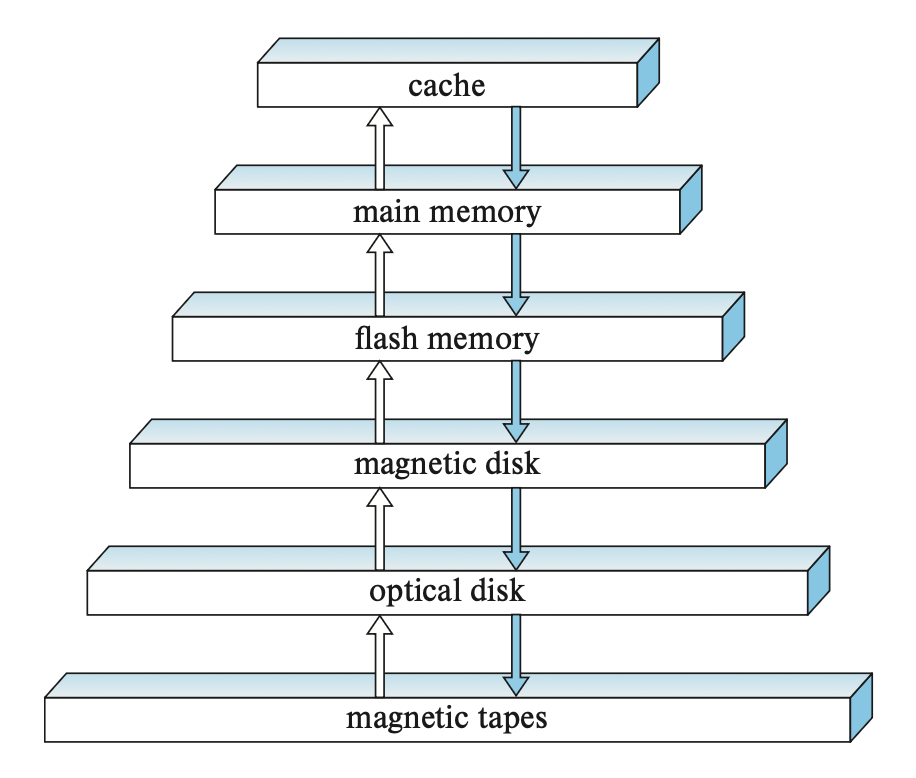
primary storage

cache:

Fastest speed, highest cost

main memory:

Data-related operations (executed by machine instructions) are all performed on the main memory.
Main memory is volatile; when power is cut off or the system crashes, the contents in the main memory are lost.

secondary storage / online storage

flash memory:

Non-volatile, meaning data will not be lost in the event of a power outage or failure
Examples: USB flash drives, solid-state drives

magnetic-disk storage:

Accessing data on a disk is relatively cumbersome: first, the system must move the data from the disk to a location in main memory where it can be accessed; after the system completes the specified operation, the modified data must be written back to the disk.

teriary storage / offline storage

optical storage:

Including: DVD (digital video disk), Blu-ray DVD
Optical disk jukebox

tape storage:

Generally used for backing up and storing archival data.

8.2 Storage Interfaces

Serial ATA, SATA
Serial Attached SCSI，SAS
Non-Volatile Memory Express，NVMe
storage area network,SAN
Network attached storage，NAS
cloud storage

8.3 Magnetic Disks

Physical Characteristics

Model diagram:

A disk consists of the following parts:

A set of platters
A drive motor and spindle
The disk surface is divided into multiple tracks, and tracks are further divided into multiple sectors
Above the surface of each platter, there is a read-write head, which is mounted on a disk arm
The read-write heads on all platters move together, so the i-th track of all platters is called the i-th cylinder
A disk controller connects the computer system and the disk drive. It accepts read/write commands for a specific sector and then initiates the operation.

Performance Measures

Access time: The period from initiating a read/write request to the start of data transmission, including:
- Seek time: The time required to locate the specified track
  - Average seek time: Assuming all tracks have the same number of sectors, the average seek time = 1/3 * worst-case seek time
- Rotational latency: The time to wait for the read/write head to find the specified sector
  - Average latency: Generally equal to the time required for half a rotation
Data transfer rate: The speed at which data is retrieved or stored.
- Disk I/O requests are typically initiated by the file system or directly by the database system.
- The request includes the address to be referenced, i.e., the block number (a “block” is the logical unit for storage allocation and retrieval).
- Requests can be categorized into sequential access mode and random access mode.
  - Sequential access: Consecutive requests target consecutive block numbers, usually on the same or adjacent tracks.
  - Random access: Consecutive requests target random block numbers, and performance can be measured in I/O operations per second (IOPS).
Mean time to failure (MTTF): The average time a system can run continuously without failure, used to measure disk reliability.

8.4 Flash Memory

Flash memory is divided into two types: NOR flash and NAND flash.

When reading data from flash memory, an entire page (typically 4 KB) must be read.

Solid-state drives (SSDs) are built on NAND flash memory and provide the same block-oriented interface as disks.

When performing a write operation, the data must first be erased and then rewritten, and this erase operation must be carried out simultaneously across multiple pages. Each flash memory page has a maximum number of erase cycles; once this limit is exceeded, the page can no longer be used to store data.

In addition to being limited by the relatively slow erase speed, the performance of flash memory is also constrained by the update speed of mapping logical page numbers to physical page numbers.

To extend the lifespan of flash memory, it employs a wear leveling mechanism: physical pages that have been erased many times are assigned “cold data,” which is data that is rarely updated, while physical pages with fewer erase cycles are assigned “hot data,” which is frequently updated. The above operations are all implemented by a software layer called the flash translation layer.

The performance of flash memory is typically measured by the following indicators:

number of random block reads per second
data transfer rate
number of random block writes per second

8.5 RAID

redundant arrays of independent disks

Improvement of Reliability via Redundancy

Improving reliability through redundancy means storing redundant information that is generally not needed but can be used to recover lost information after a hard drive failure.

Mirroring/Shadowing:

The simplest implementation method
Duplicates every hard drive
MTTF must consider the mean time to repair, which is the time required to recover data from a failed hard drive, and the mean time to data loss.

Improvement in Performance via Parallelism

Improve performance by supporting parallel access to multiple hard drives.

Use data striping to increase transfer rates.

Bit-level striping: Divides byte data across multiple hard drives into bits.
Block-level striping: Treats a group of hard drives as a single large hard drive, assigning each block a logical number (starting from 0). The i-th logical block is placed on the ⌊ $\frac{i}{n}$ ⌋-th physical block of the (i mod n) + 1-th hard drive.

RAID Levels

Combining hard disk striping and parity blocks

Divide the blocks in the RAID system into multiple groups, each group has a parity block, where the i-th bit is the result of XOR operation on the i-th bit of all blocks in the group.
If a block in the group loses data due to a failure, the data of that block can be recovered by performing XOR operation on the remaining blocks plus the parity block.
When data in any block is updated, the parity bit must be recalculated and the result written to the parity block.

Based on the technology described above, we classify it into multiple RAID levels:

RAID 0: Block-level striping
RAID 1: Disk mirroring + block-level striping
RAID 5: Block-interleaved distributed parity
RAID 6: P + Q redundancy, similar to RAID 5, but uses an additional disk to store error-correcting codes, allowing for the failure of two disks.

Hardware Issues

Latent Failure / Bit Rot:

Even if data is written correctly, it may later become unreadable in that sector.

Scrubbing:

When the disk is idle, every sector of each hard drive is read. If a sector is found to be unreadable, data is recovered from the other drives and written back to that sector. If the sector has physical damage, the logical sector address must be remapped to a different physical sector.

Hot Swapping:

Without powering off, remove the faulty hard drive and replace it with a new one.

Choice of RAID Level

When selecting a RAID level, the following factors need to be considered:

The monetary cost of additional hard drive storage requirements
Performance requirements in terms of I/O operations per second
Performance during hard drive failure
Performance during data reconstruction (rebuilding data from a failed drive onto a new one)

A brief overview of the applicable scenarios for different RAID levels:

RAID 0: Suitable for a few scenarios where data security is not critical but high performance is needed
RAID 1: Ideal for applications that store log files (due to its best write performance) and have high demands for random I/O
RAID 5: Suitable for situations where data is frequently read but writes are infrequent
RAID 6: Offers the best reliability, making it suitable for scenarios where data security is extremely important

8.6 Disk-Block Access

Some techniques to improve access speed by reducing (random) access times:

buffering: Data blocks read from the hard disk are temporarily stored in the memory buffer to meet future access demands.
read-ahead: When accessing a certain data block on the disk, a continuous group of blocks located on the same track will be read into the buffer simultaneously.
scheduling: disk-arm scheduling algorithm, Try to sort all accesses in order of track to increase the number of accesses that can be processed, similar to the elevator algorithm.
file organization: Organize the blocks in the hard disk according to how we expect to access them.
- fragmented: Data blocks are distributed across multiple hard drives.
non-volatile write buffers:
- Using non-volatile random-access memory (NVRAM) to accelerate hard disk write operations
- When a database system or operating system initiates a request to write a block to disk, the disk controller writes the block to a non-volatile write buffer and immediately informs the operating system that the write operation is complete; afterward, the disk controller writes the data to the disk in a manner that minimizes disk arm movement.

Chapter 9 Database Storage Structures

9.1 File Organization

A database is mapped to multiple different files.

A file contains a sequence of records from the database, and these records are mapped to disk blocks (or pages), which serve as the basic units for storage allocation and data transfer.

For the convenience of subsequent discussion, we agree that:

A record must not be larger than the size of a disk block (while a disk block may contain multiple records).
Each record can only be contained within one disk block.

Pages

A page can contain different types of data (tuples, indexes, etc.), but most systems do not allow mixing multiple types of data within a single page.

Each page has a unique identifier (called a page ID). If the database is a single file, the page ID is the file offset. Most DBMSs provide an indirection layer that maps page IDs to file paths and offsets, with the storage manager handling this translation.

There are generally three types of page sizes:

Hardware page: typically 4KB
OS page: 4KB
Database page: 1-16KB

The storage device guarantees that the size of an atomic write is equal to the hardware page size.

Records

Fixed-Length Records

A very simple method is to directly allocate the maximum byte space for variable-length types. However, this approach leads to the following issues:

Some records may cross block boundaries, meaning certain records are located within two blocks. Accessing such records requires two read/write operations.
- Solution: Only allocate records that can fit entirely within each block, and simply ignore the extra space.
It is difficult to delete such records because after deletion, the space needs to be filled with other records or simply ignored.

For the issue of record deletion, the following solutions exist:

Move all records after the deleted record forward to fill the space left by the deleted record.
- This method requires moving a large number of records and is inefficient.
Directly fill the space of the deleted record with the last record.
- This may lead to additional block accesses.
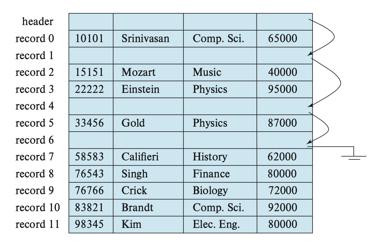
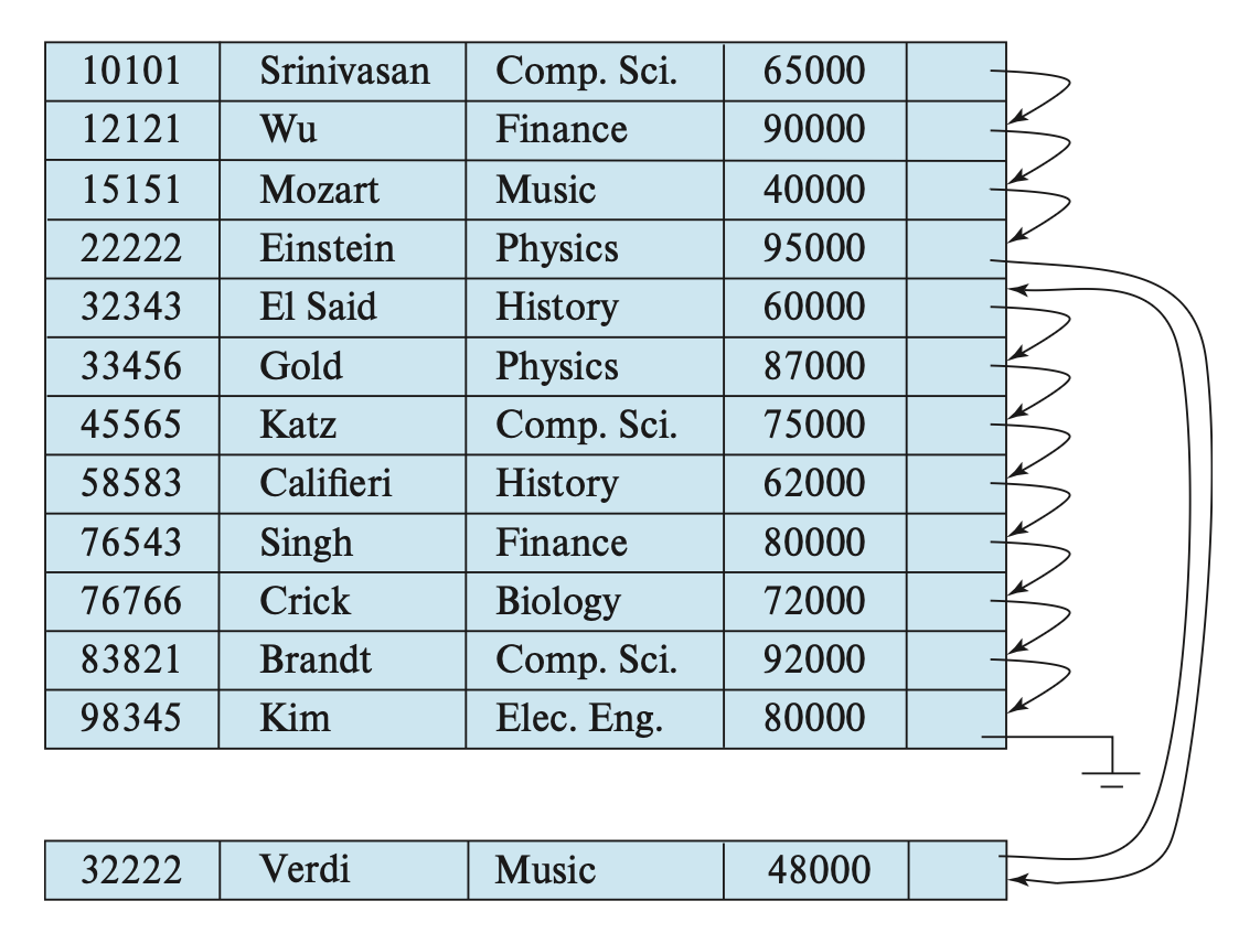
Temporarily leave the space of the deleted record open and wait for subsequent insertions.
- At the beginning of the file, we allocate some specific bytes as the file header, which contains information about the file.
- Here, we only care about the address of the first deleted record (where space is freed). On this record, we record the second deleted free record.
- These deleted records form a linked list, commonly referred to as a free list.

Variable-Length Records

How to represent a single record so that extracting a single attribute is relatively easy, even if the attribute is of variable length

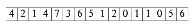
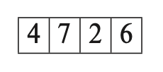
Variable-length attributes are represented in two parts: fixed-length information (offset (starting position of the data) + length (size of the variable-length attribute)), and the variable-length attribute value. The structure diagram is as follows:

This record first stores the fixed-length information of three variable-length attributes, followed by a fixed-length attribute value, and finally the variable-length attribute values.

Between the fixed-length attribute value and the variable-length attribute values, there is a set of zeros called the null bitmap, which is used to record whether an attribute value is null. If an attribute value is null, the corresponding bit in the null bitmap is set to 1.

Each page has a header that contains metadata related to the page’s content, including: page size, checksum, DBMS version, etc.

How to store variable-length records within a block to make it easier to extract records from the block

We use a slotted-page structure to organize records within a block, as shown in the following figure:

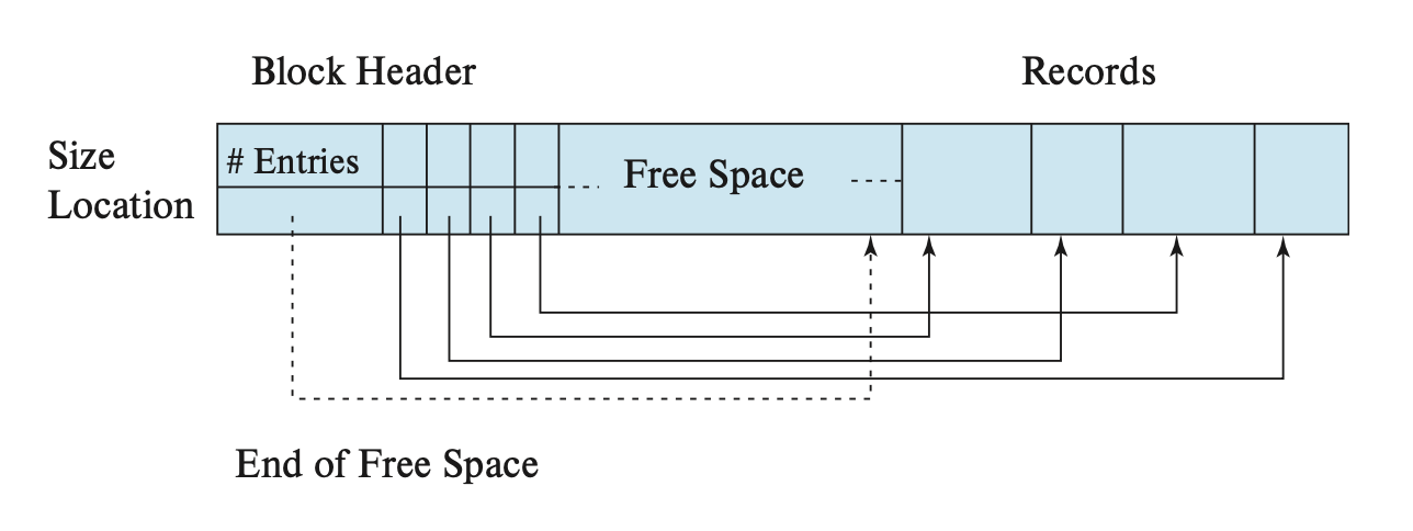
Each block begins with a header that contains the following information:

The number of records in the header
The end position of free space within the block
An array containing the position and size of each record

When a record is inserted, space is allocated at the end of the free space, and the record’s position and size are recorded in the header.

When a record is deleted, the space it occupies is released, and the corresponding entry in the header array is marked as deleted (for example, by setting its size to -1).

Additionally, all records before the deleted record need to be moved to free up space equivalent to the size of the deleted record. The cost of moving is not significant because the block size is limited to a certain range.

This slotted-page structure requires that pointers do not directly point to records but instead point to the corresponding header array elements, which contain the record’s position. This indirection helps avoid fragmentation within the block.

Drawbacks include:

Internal fragmentation within the page: Deleting certain records can create gaps in the page’s internal space.
Due to the block-oriented nature of non-volatile memory, updating a record requires fetching the entire block.
Updating multiple tuples may require jumping between different locations, which can make I/O very slow.

The DBMS is responsible for tracking and interpreting these bytes as attributes. It wants to ensure that tuples are word-aligned, so that the CPU does not encounter abnormal behavior or perform extra work when accessing data. There are two ways to achieve this:

Padding: Adding empty spaces after attributes to ensure that tuples are word-aligned.
Reordering: Changing the order of attributes in the physical layout to ensure they are aligned.

A tuple is essentially a byte sequence (which may not be contiguous). The DBMS needs to interpret this sequence as attributes and their corresponding values.

Tuple header (i.e., metadata of the tuple)
Tuple data: the actual data about the attributes
Unique identifier: mostly page_id + (offset or slot)

The organization of records within a file:

Heap file organization: Any record can be placed anywhere in the file without considering order. A relation can be stored in one or more files.
Sequential file organization: Records are stored in order based on the value of each record’s “search key.”
Multitable clustering file organization: Records from different relations are stored in the same file to reduce the cost of join operations.
B+ tree file organization: Maintains the order of records even when insert, delete, and update operations change the record order. This content will be introduced in the next lecture.
Hash file organization: A hash function is computed based on certain attributes to determine which block a record should be placed in.

Heap File Organization

In a heap file organization, a record can be placed at any position in the file. However, once its position is determined, the record generally cannot be moved.

When inserting records into a file, a strategy of always appending them to the end of the file can be adopted.

For record deletion, we need to consider utilizing the space freed by deleted records to store new records, maximizing space usage.

Most databases use a data structure called a free-space map to efficiently locate free space.

This data structure is typically represented as an array, where each element corresponds to a block, and its value indicates the proportion of free space in that block.
To find a block that can store a new record, the database needs to scan the free-space map to locate a block with sufficient free space.
If no such block exists, a new block must be allocated for the relation.

Suppose each element of the free-space map is 3 bits in size. When an element has a value of 7, it indicates that at least 7/8 of the corresponding block’s space is free.

For large files, such scanning is still too time-consuming. In this case, we can create a second-level free space map, where each element corresponds to the maximum value of 100 elements in the primary (first-level) free space map. For even larger files, additional levels of free space maps can be created.

Continuing with the example above, if one element in the second-level free space map corresponds to four elements in the first level, its content would be:

If the free space map were written to the hard drive with every update, the cost would be too high. Therefore, the free space map is typically written periodically. However, this means the free space map on the hard drive may become outdated, and accessing such a map could lead to errors.

Page Location Methods
Linked List: The header page contains pointers to free pages and data pages. If the DBMS needs to find a specific page, it must sequentially scan the list of data pages until it finds the required page.
Page Directory: The DBMS maintains a special page called the page directory to track the locations of data pages, the amount of free space on each page, lists of free/empty pages, and page types. Each database object has a corresponding entry in the page directory.

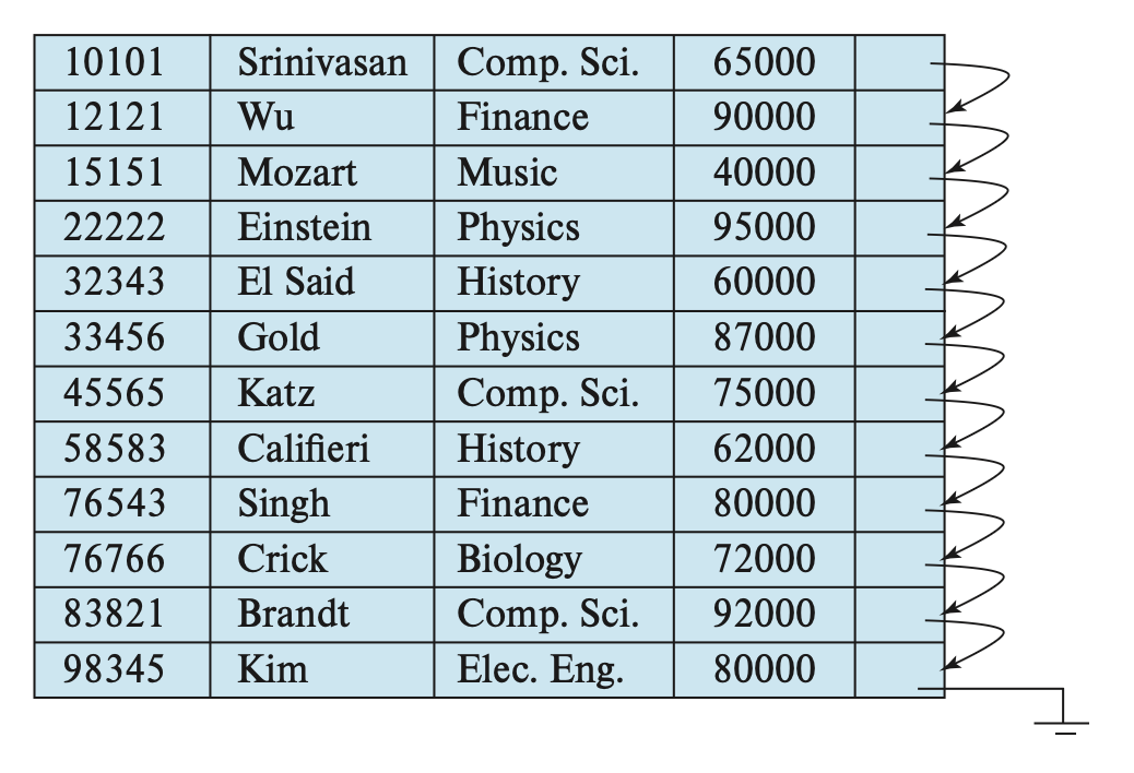
Sequential File Organization

Sequential files are used to efficiently process ordered records, and they are implemented based on a search key.

To retrieve records more quickly, we link these records using pointers. Additionally, to minimize the number of block accesses, we physically store the records in the order of the search key.

Maintaining the order of records at the physical level is difficult because records can be inserted and deleted at any time.

For deletion, it can be handled by moving pointers.
For insertion, the following rules must be followed:
- Before inserting a record by its search key, find the position of the record in the file.
- If there is a free record located in the same block as the record, place the new record directly in that free space. Otherwise, insert the new record into an overflow block. In both cases, the corresponding pointers need to be adjusted to maintain the order of the search keys.

As time passes, the correlation between the search key order and the physical order gradually diminishes, making sequential processing less effective. At this point, we need to reorganize the file, but such an operation is costly and must be performed when the system load is low. The frequency of reorganization depends on the frequency of record insertions.

Multitable Clustering File Organization

In some cases, it is more useful to store records from multiple relations within a single block.

Multitable clustering file organization is a file organization that stores related records from multiple relations within a single block. The clustering key is the attribute used to define which records are stored together.

Although this file organization speeds up specific join query operations, it can affect the performance of processing other types of queries, so use it with caution.

Partitioning

Many databases allow partitioning a relation into multiple smaller relations, storing them separately, thereby reducing the cost of certain operations by decreasing the size of the relation.

We can also divide a relation into multiple parts and store different parts on different storage devices—for example, placing frequently used parts on SSDs and less frequently used ones on disks.

9.2 Data-Dictionary Storage

We generally refer to this “data about data” as metadata. Such metadata is stored in a structure called a data dictionary or system catalog.

The system must store the following metadata:

Names of relations
Attribute names for each relation
Domains and lengths of attributes
Names and definitions of views
Integrity constraints

In addition, many systems also store data about users, including: usernames, default schemas of users, passwords of authorized users, and other information.

Some databases may also store statistical and descriptive data about relations and attributes, such as the number of tuples in each relation, the number of distinct values for each attribute, and so on.

The data dictionary may also record the storage organization of relations (heap, sequential, hash, etc.) and the location where the relation is stored. If a relation is stored in an operating system file, the dictionary records the file name containing the relation; if the database stores all relations in a single file, the dictionary uses data structures like linked lists to record the blocks where the records of each relation are located.

We also need to store information related to indexes (which will be covered in detail in the next lecture), including: index names, the names of the indexed relations, the attributes defining the index, and the type of index structure.

This metadata essentially forms a miniature database. Therefore, we can store it within a relation in the database, simplifying the overall system structure and leveraging the fast access capabilities of the database.

The relationships in the stored data dictionary are denormalized to ensure faster access.

When a database system needs to retrieve data from a certain relationship, it must first query this relationship called Relation_metadata to find the location and storage organization of the relationship before it can retrieve the records.

Since these system metadata are frequently accessed, most databases read them into an in-memory data structure for efficient access, and this step is performed as part of the database startup process.

9.3 Database Buffer

A major goal of database systems is to minimize the number of data block transfers between the disk and memory. The buffer is the portion of main memory used to store copies of disk blocks, and the allocation of buffer space is managed by the buffer manager.

Buffer Manager

When a program within the database system requires a data block from the hard disk, it sends a request to the buffer manager.

If the data block is already in the buffer, the buffer manager sends the address of the block in main memory to the requester.
If not, the buffer manager first allocates space for the block in the buffer. If necessary, it may discard some existing blocks, but if these blocks have been modified since they were last written from the hard disk to main memory, they must be written back to the hard disk first. Then, the buffer manager reads the required block from the hard disk into main memory and sends the main memory address to the requester.

The buffer pool consists of an array of fixed-size frames. When the DBMS requests a page, the buffer manager first checks whether the page already exists in a memory frame; if not found, it reads/copies the page from disk to a free frame.
The buffer manager implements a write-back strategy, meaning that modified dirty pages are temporarily stored in the buffer rather than being immediately written to disk.
The buffer pool can be used for: tuple storage and indexing, sorting and join buffers, query and dictionary caches, maintenance and log buffers.
The buffer pool must maintain some metadata to ensure efficient and correct execution: page table, dirty flag, pin/reference counter.

If there is no extra space in the buffer, a data block must be evicted, meaning it is removed before reading in a new data block. The specific eviction strategy will be introduced in the next section.

Sometimes this situation occurs: when the main memory is reading/writing a certain data block, another concurrent process evicts this data block and replaces it with a different one, which can lead to reading incorrect data or corrupting the data.

Therefore, it is necessary to ensure that the data block will not be evicted before reading data from the buffer. Specifically, the process performs a “pin” operation on the data block to prevent the buffer manager from evicting it. Once the read operation is completed, the process performs an “unpin” operation, allowing the data block to be evicted.

When designing a database, care must be taken not to pin too many blocks; otherwise, the database will not function properly.

If multiple processes are simultaneously reading a certain data block in the buffer, each process will perform pin and unpin operations, and the data block can only be evicted after all processes have performed the unpin operation.

A simple approach is to maintain a pin count. Each pin operation increments this count by 1, and each unpin operation decrements it by 1. The data block can only be evicted when this count equals 0.

The process of adding or removing a tuple from a data block may require moving the contents of the data block. During this time, no other process should read the contents of the data block; otherwise, data inconsistency may occur.

To achieve this, the buffer manager provides a locking system that allows database processes to acquire a shared lock or an exclusive lock on a data block before accessing it. Once the access is complete, the lock is released.

Any number of processes can simultaneously hold a shared lock on the same data block.
At any given time, only one process is allowed to hold an exclusive lock on a data block. When a process holds an exclusive lock, other processes cannot use a shared lock. Therefore, an exclusive lock can only be granted to a process when no other process holds a lock on the data block.
If a process requests an exclusive lock on a data block that already has a shared lock or an exclusive lock, the request will wait until all previous locks are released.
When a data block is not locked or already has a shared lock, a shared lock request from a process will be accepted. However, if the data block has an exclusive lock, the request must wait until the lock is released.

Specific locking operations:

Before performing any operation on a data block, the process must first pin the data block, then acquire a lock on it. This lock will be released before the unpin operation is executed.
Before performing any operation on a data block, the process must first pin the data block, then acquire a lock on it. This lock will be released before the unpin operation is executed.
Before reading a data block, the process must acquire a shared lock. Once the reading is complete, the process must release the lock.
Before updating a data block, the process must acquire an exclusive lock. Once the update is complete, the process must release the lock.

Forced output: Write the data block from the buffer back to the hard disk to ensure the consistency of specific data on the hard disk.

Buffer-Replacement Strategies

The goal is to minimize access to the hard disk.

Least Recently Used (LRU): Replaces the data block that has not been referenced for the longest time.

Clock: An approximate implementation of LRU. It uses a reference bit instead of a timestamp. When a page is accessed, its reference bit is set to 1. These pages are placed in a circular buffer, and a clock hand scans through them in order: it checks whether the reference bit of the page pointed to by the hand is 1; if so, it sets it to 0; otherwise, it evicts the page.

Compared to operating systems, database systems can predict future access patterns more accurately. A user’s request to a database system consists of multiple steps, and the database system can read these steps to determine in advance which data blocks will be needed. Therefore, database systems may adopt a replacement strategy better than LRU.

Toss-immediate: Once a tuple’s data block has been processed, the main memory no longer needs this block, even if it was recently used. When the last tuple in the data block has been processed, the buffer manager releases the space occupied by this block.

Most Recently Used (MRU) strategy: The most recently used block will be the last to be referenced again, while the least recently used block will be the next one to be referenced.

An ideal database replacement strategy requires knowledge of database operation-related information, including both currently executing and future operations. However, no known strategy can handle all scenarios. In fact, most database systems use LRU, despite its issues: it only records the last access time of a page, without tracking the frequency of page accesses.

LRU-K: Tracks the history of the previous K references (as timestamps) and calculates the intervals between subsequent accesses. This history is used to predict when a page will be accessed next. However, this approach incurs higher storage overhead. Additionally, an in-memory cache must be maintained for recently evicted pages to prevent them from being constantly evicted.

Localization: The DBMS selects which page to evict based on individual queries or transactions, thereby minimizing the pollution of the buffer by each query.

Priority Hints: The buffer can determine which pages are important based on the context of query execution, using information from transactions about each page.

Reordering of Writes and Recovery

Database buffers allow write operations to be completed in main memory and then output to the hard disk after some time, which may cause the order of output to the hard disk to differ from the order in which the write operations were executed. Additionally, the file system may also reorder write operations, but this can lead to inconsistencies in hard disk data in the event of a system crash.

Early file systems performed a file system consistency check upon system restart to ensure data structure consistency. If inconsistencies were found, additional steps were required to restore consistency. However, these checks resulted in long delays.

If the file system could write updates to metadata in a carefully chosen order, many inconsistencies could be avoided. However, doing so would render some optimization strategies ineffective, such as disk arm scheduling, thereby affecting update efficiency.

Modern file systems use a hard disk to store a log of write operations sorted by execution order. Such a hard disk is called a log disk. Once a write operation is completed, the record is removed from the log disk.

File systems that support a log disk are called journaling file systems. These systems allow data and logs to be stored on the same hard disk, reducing costs at the expense of performance. Since no consistency check is required, they enable faster system restarts.

Optimization methods for the buffer pool:

Multiple buffer pools: The DBMS can maintain buffer pools for different purposes. These buffer pools can adopt customized strategies based on the stored data to reduce latch contention and improve locality. Object IDs and hashing are two common methods for mapping pages to specific buffer pools:
- Object ID: Extended from record IDs, these IDs maintain mappings to achieve fine-grained control over buffer pool allocation, but they incur additional storage overhead.
- Hashing: The DBMS hashes the page ID to select a specific buffer pool.
Pre-fetching: When the first set of pages is processed, the second set can also be pre-fetched into the buffer pool. The advantage lies in sequential scanning.
Scan sharing (synchronized scans): Query cursors can reuse data retrieved from storage or computation.
Buffer pool bypass: Sequential scan operators (or when reading a large contiguous block of pages) do not store the fetched pages in the buffer pool to avoid overhead. This is suitable for temporary data.

9.4 Column-Oriented Storage

row-oriented storage: Place all attributes of the tuple in a single record.

column-oriented storage: Store each attribute in the relationship separately.

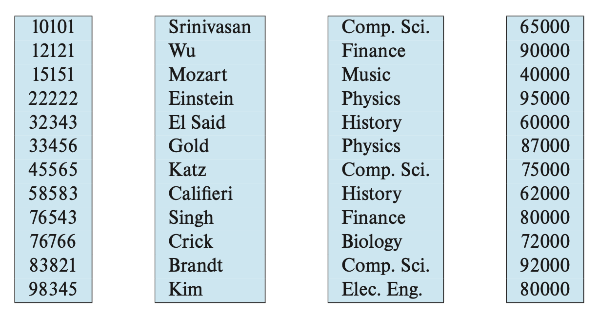
This column-oriented storage is suitable for data analysis queries, which need to process multiple rows in a relation but typically access only a subset of attributes.

Reduces I/O operations
Improves CPU cache performance
Enhances compression capabilities
Enables vector processing

Column-oriented storage also has the following drawbacks:

High cost of tuple reconstruction

Tuple Reconstruction Methods
Fixed-Length Offsets: We place the value from one column and the value from another column at the same offset into the same tuple. Therefore, each individual value in a column must have the same length.
Embedded Tuple IDs: For each attribute in a column, the DBMS stores a tuple ID associated with it. Additionally, the system stores a mapping that tells it how to jump to each attribute with that ID. This method is not recommended due to its high storage overhead (storing a tuple ID for each attribute entry).

High cost of tuple deletion and updates
High cost of decompression

ORC and Parquet are columnar file representations used in many big data processing applications. ORC divides a sequence of tuples occupying several hundred MB into a columnar representation called a stripe, and an ORC file contains multiple such stripes. The following figure shows some details of the ORC file format:

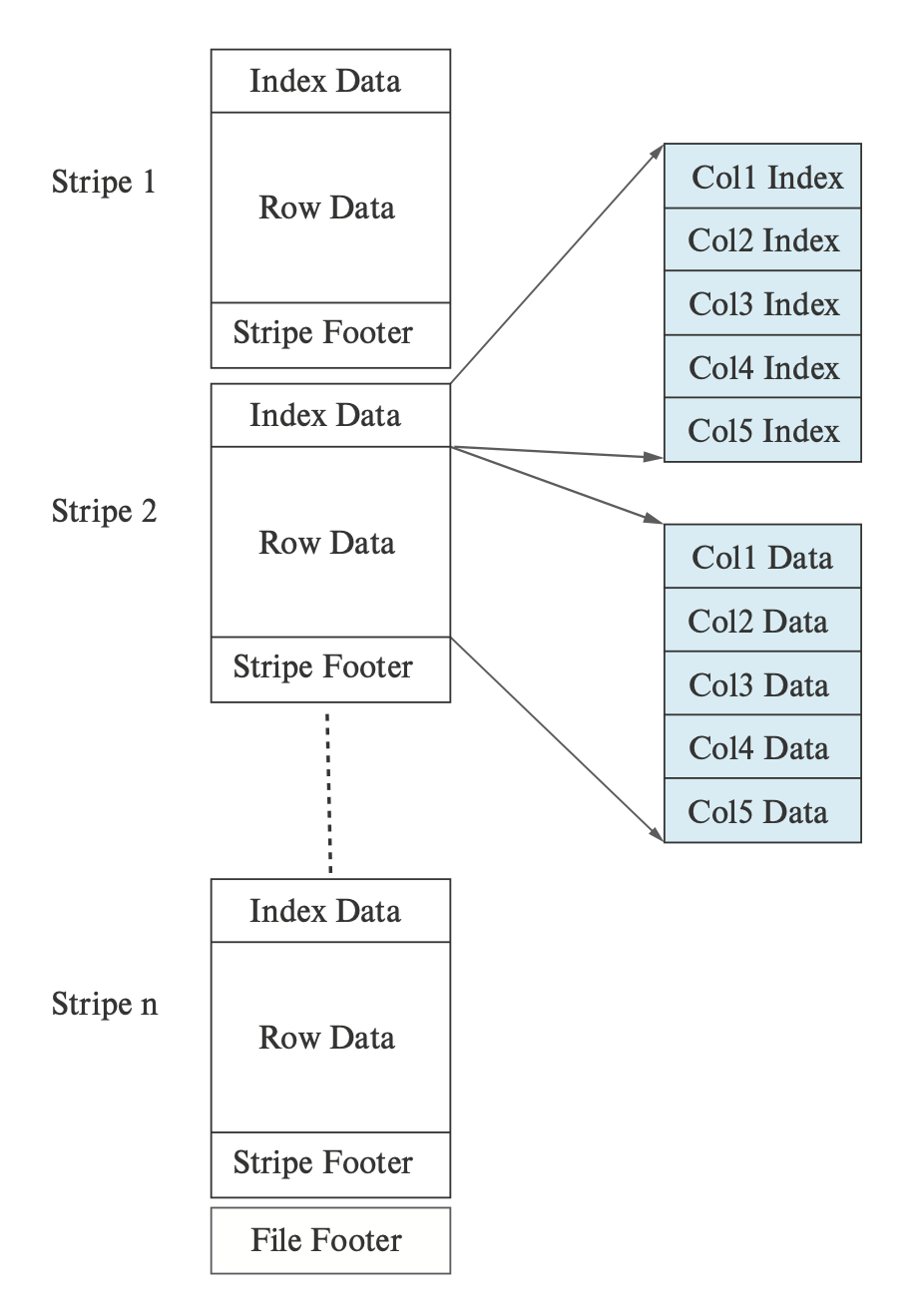
Each stripe contains an index data, row data, and a stripe footer. ORC files also have a file footer, but we will not consider these two “footers.”
Row data contains the compressed sequence values of each column.
Index data is used for fast access to the required tuples.

9.5 Storage Organization in Main- Memory Databases

A main-memory database refers to a database where all data resides in memory, used to optimize performance. A main-memory database may retain direct pointers to records in memory, allowing a record to be accessed through a single pointer traversal, which is highly efficient.

If the main memory uses a column-oriented storage method, all values of a particular column are stored in contiguous memory locations. However, when records are appended to a relation, to ensure contiguous space allocation, the space for existing data needs to be reallocated. To avoid this overhead, the logical array of a column is divided into multiple physical arrays, and an indirection table is used to store pointers to all physical arrays, as shown below:

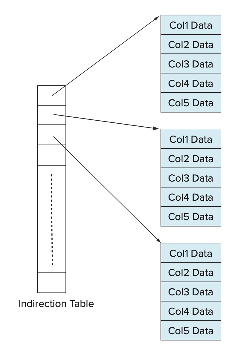
Chapter 10 Indexing

Indices are composed of organized or sorted columns in a table, used to efficiently access database content. A DBMS ensures that the table content and indices are logically synchronized.

The following two basic types of indices are commonly used in databases:

Ordered indices: based on sorted values
Hash indices: based on the uniform distribution of values across buckets, where the bucket a value is assigned to is determined by a hash function

Relevant metrics:

Access type: includes finding records with specified attributes or attribute value ranges
Access time: the time required to find a single or multiple data items
Insertion time: includes the time needed to find the correct position for inserting new data and updating the index structure
Deletion time: includes the time needed to find the data item to be deleted and updating the index structure
Space overhead: the additional space occupied by the index structure; if this space is not large, it is worth trading for performance improvement

A single attribute or multiple attributes used to locate records in a file are called search keys, and each index corresponds to a specific search key.

10.1 Ordered Indices

If the order within the file is defined by the search key, the corresponding index is called a clustering index or primary index, and the corresponding file is referred to as an index-sequential file.

For indexes where the search key order differs from the file order, we call them nonclustering indexes or secondary indexes.

Dense and Sparse Indices

An index entry or index record consists of a search key value and a pointer to one or more records that have the same value as the search key.

This pointer includes the identifier of the disk block and the offset within the disk block to identify the specific record within the block.

Sequential indexes can be divided into the following two categories:

Dense index: There is a corresponding index entry for every search key value in the file. In a dense clustered index, the index record contains the search key value and a pointer to the first record with that search key value, while the remaining records with the same search key value are stored sequentially after this first record.

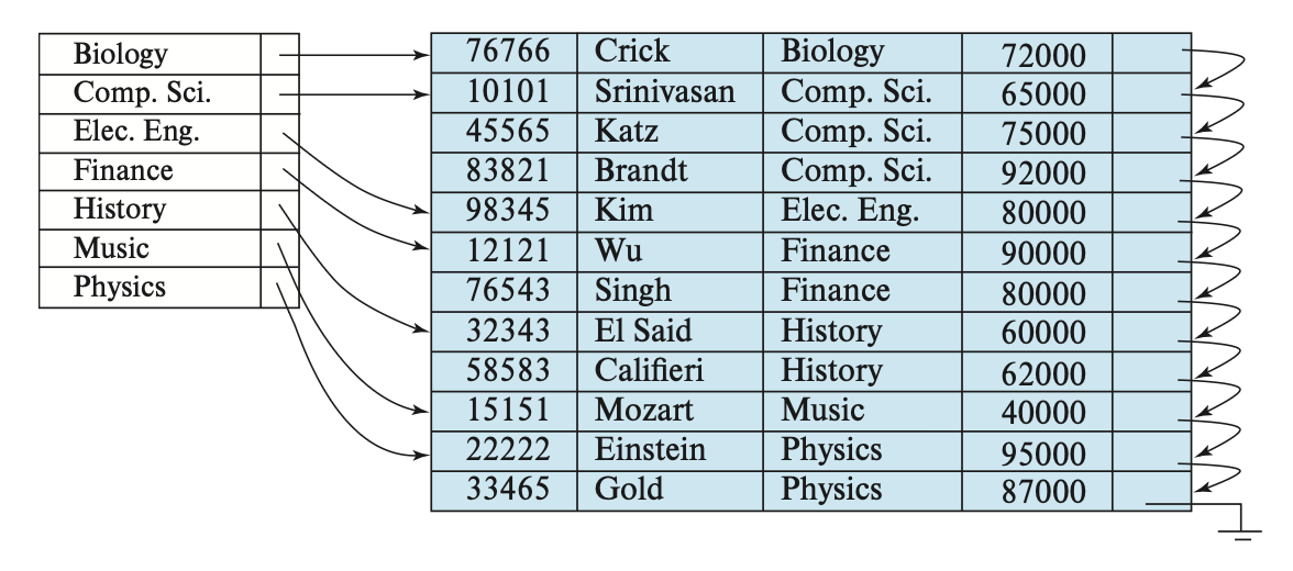
Sparse Index: Only some search key values in the file have corresponding index entries.
- In this case, only clustered indexes are allowed. Each index entry contains a search key value and a pointer to the first record with that search key value.
- To locate a record, find the index entry corresponding to the largest search key value that is less than or equal to the target search key value. Then, starting from that record, follow the pointers in the file until the desired record is found.

The main cost of processing database requests is the time required to bring data blocks from the hard disk to main memory.

Multilevel Indices

When the index is very large, the process of searching the index becomes particularly time-consuming. To address this issue, we can treat the index as a record in a file and build a sparse index for it. The original index is called the internal index, while the newly constructed index is referred to as the external index, as shown below:

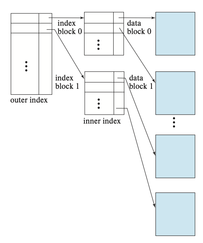
To find a specific record, we first perform a binary search on the outer index to locate the record with the largest search key value that does not exceed that of the target record. This record corresponds to a pointer to an inner index block. Then, within that inner index block, we find the record with the largest search key value that does not exceed the target record’s search key value, which corresponds to a pointer to a file block containing the record we are looking for.

When the index becomes very large, we can use multiple levels of indexing, known as multilevel indices. Compared to using only binary search, searching for records on multilevel indices can significantly reduce I/O operations.

Index Update

Insertion

First, the system locates the insertion point for the record using the search key.
Dense index
- If the search key value does not appear in the index, the system inserts a new index entry with that search key at the appropriate position.
- Otherwise, if the index entry stores pointers to all records with the same search key, the system adds a pointer to the new record in the index entry.
- Otherwise, the index only stores a pointer to the first record with that search key, and the system inserts the new record after the records with the same search key value.
Sparse index:
- Assume the index stores one entry per block. If the system creates a new block, it inserts the search key value obtained from the new block into the index.
- If the search key value of the new record is the smallest within the block, the system updates the index entry to point to that block; otherwise, no change is made.

Deletion

First, the system needs to locate the record to be deleted.
Dense index:
- If the deleted record is the only record corresponding to the search key value, the system will delete the corresponding index entry.
- Otherwise, if the index entry stores pointers to all records with the same search key, the system will delete the pointer to the deleted record.
- Otherwise, the index only stores a pointer to the first record with that search key, and the system will update the index entry to point to the next record.
Sparse index:
- Assume that the index stores only one index entry per block, and the index entry points to the first record in that block.
- After deleting a record, the index usually does not need to be modified.
- However, if the deleted record happens to be the first record in the block, then the corresponding index entry for that block needs to be updated to point to the next record in the block.
- If the block becomes empty after deletion, the system will delete the corresponding index entry; if the database also reclaims the empty block, it may be necessary to adjust the index information of adjacent blocks accordingly.

Secondary Indices

Secondary indexes can also be dense indexes, where the index entries correspond to all search key values and contain pointers to all records.

A secondary index on a candidate key resembles a dense clustered index, but the difference is that the set of records pointed to by consecutive values in the index is not stored in order.

If multiple records in a relation have the same search key value, such a search key is called a nonunique search key.

One method for implementing a secondary index on a nonunique search key is to have the pointers in the secondary index not directly point to records, but instead let each pointer point to a bucket that contains pointers to the file. The following figure illustrates such a structure:

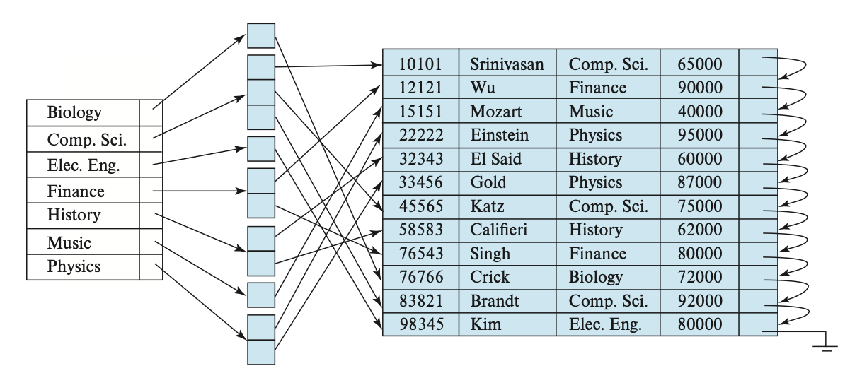
The drawbacks are:

Index access time becomes longer
If there are few duplicate search keys, a lot of space will be wasted

Since the order of secondary search keys differs from the order of physical search keys, attempting to scan the file in the order of secondary search keys results in reading each record as if reading every block on the hard drive, which is quite slow.

In general, secondary indexes improve performance when querying using keys other than the clustered index’s search key, but they introduce additional overhead for database modifications.

10.2 B+ Tree Index Files

The main disadvantage of indexed sequential file organization is that as the file size grows, the performance of index lookup and sequential data scanning decreases.

The B+ tree, a widely used index structure, ensures efficiency even when data is inserted or deleted.

Structure

A B+ tree is a balanced tree, meaning that all paths from the root node to the leaf nodes are of equal length.

The following figure shows the content of a node in a B+ tree, which contains $n-1$ search key values $K_1, K_2, \dots, K_{n-1}$ and n pointers $P_1, P_2, \dots, P_n$ , with the search key values sorted.

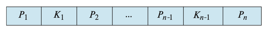
First, consider the structure of leaf nodes.

For $i = 1, \dots, n - 1$ , $P_i$ points to the file record (tuple) with search key value $K_i$ ; while $P_n$ points to the next leaf node to enable efficient sequential file processing. A leaf node contains at least $\lceil \dfrac{n-1}{2} \rceil$ values.

The nonleaf nodes (sometimes called internal nodes) of a B+ tree form a multi-level (sparse) index over the leaf nodes.

The structure of nonleaf nodes is similar to that of leaf nodes, except that their pointers all point to nodes within the tree.
The number of children for each nonleaf node (excluding the root) ranges from $[\lceil \dfrac{n}{2} \rceil, n]$ , while the number of children for the root node ranges from $[2, n]$ .
The number of pointers in a node is called the fanout.
If a node contains $m (m \le n)$ pointers, pointer $P_i$ points to the subtree whose search key values are less than $K_i$ and not less than $K_{i-1}$ .
The value $K_i$ in an internal node is the first search key value of the first leaf node in the subtree pointed to by $P_{i+1}$ .

If there are duplicate search keys, most database systems combine an additional primary key $A_p$ with the search key attribute $a_i$ to form a unique composite search key $(a_i, A_p)$ .

Quries

range queries: Searching for records corresponding to search key values within a specific range $[lb, ub]$ on a B+ tree

First, perform an operation similar to $find(lb)$ to locate the starting leaf node; then traverse the leaf nodes, collecting records whose search key values fall within the range, until a search key value greater than $ub$ is encountered, or there are no more records to traverse; finally, return the collected records $resultSet$

Cost of querying a B+ tree index:

If there are a total of $N$ records, the path length of the B+ tree does not exceed $\lceil \log_{\lceil n/2 \rceil} N\rceil$
Generally, the node size is consistent with the hard disk block size (approximately 4KB)
When traversing to the bottommost leaf node, querying a unique search key value requires one additional random I/O access

For non-unique search keys, to retrieve all records under a given search key value $v$ , the process $findRange(lb, ub)$ can be used, where $lb = (v, -\infty), ub = (v, \infty)$ , and $-\infty, \infty$ refer to the minimum and maximum primary key values $A_p$ , respectively.

Updates

The process of updating records can be broken down into: deleting the old record, then inserting the updated record.

Insertion: Use the $find()$ function to locate the position of the leaf node for insertion, then insert the search key value, ensuring that the search keys within the leaf node remain in order.
Deletion: Also use the $find()$ function to locate the search key value to be deleted. If there are multiple identical search key values, all of them must be found and deleted. After deletion, all items to the right of the deleted search key value must be shifted left to ensure there are no gaps between items.

Insertion

overflow: Split $L$ into two nodes, $L$ and $L_2$ . Evenly distribute the original items in $L$ between the two nodes, and copy the middle item to the parent node. Insert an item pointing to $L_2$ into the parent node of $L$ . Push the middle item up to the parent node.

Process recursively from bottom to top

Deletion

Underflow: First, attempt to merge with the sibling node; if merging fails (the number of items after merging exceeds the node capacity), then redistribute the contents of these two nodes ( $L$ and its sibling node) (more precisely, “borrow” an item from the sibling node). Delete the item in $L$ ‘s parent node that points to $L$ .

Since the deletion operation is bottom-up, the leaf node does not care which value is deleted—it only cares about whether underflow occurs. Therefore, it is possible for an item to not exist in a leaf node but still exist in an internal node.

Complexity

If the number of records is known to be $N$ and the maximum number of pointers in a B+ tree node is $n$ (meaning a node can hold at most $n-1$ search key values), then the formula for calculating the tree height is:

Best case (each node is completely full): $H_{\min} = 1 + \lceil \log_n \lceil \dfrac{N}{n-1} \rceil \rceil$
Worst case (the root node has only 2 subtrees, and other nodes have only half the maximum fanout): $H_{\max} = 2 + \lfloor \log_{\lceil n / 2 \rceil} \lceil \dfrac{1}{2} \cdot \dfrac{N}{(n-1) / 2} \rceil \rfloor$

If the search key values are inserted randomly, then on average each node is about 2/3 full; if inserted sequentially, then only half is full.

Nonunique Search Keys

By modifying the structure of the B+ tree, it can support the search, insertion, and deletion of duplicate search keys. Specifically, the following methods can be used:

Each search key value is stored only once, and a bucket (or list) of record pointers is retained for each search key value to handle non-unique search keys. This method effectively utilizes space but makes the implementation of the B+ tree more complex.
Each record stores the search key value only once. This method keeps the leaf node splitting operation unchanged. However, it makes the splitting and searching of internal nodes quite complex.

The common drawback of these two methods is that they affect the efficiency of record deletion. In the worst case, the complexity of deletion is linear with respect to the number of records. In contrast, when the search key is unique, the worst-case complexity of record deletion is logarithmic with respect to the number of records.

10.3 B+ Tree Extension

B+ Tree File Organization

B+ tree file organization: stores the actual records in the file on the leaf nodes of the B+ tree.

Since records are typically larger than pointers, the maximum number of records that can be stored in a leaf node is smaller than the number of pointers in a non-leaf node; even so, we still require that leaf nodes be at least half full.

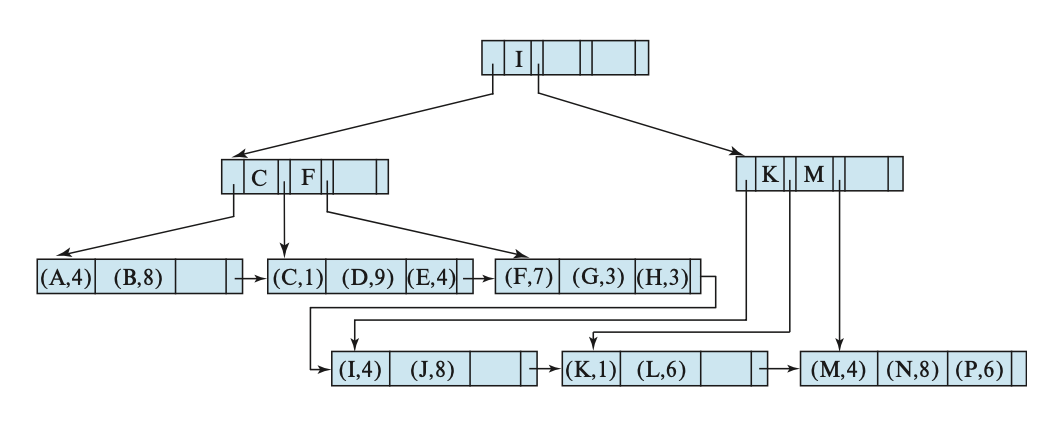
Space utilization can be improved by considering more sibling nodes during redistribution operations when splitting or merging. This approach is feasible for both leaf and non-leaf nodes. In general, if $m$ nodes ( $m - 1$ sibling nodes) are considered during redistribution, each node is guaranteed to obtain at least $\lfloor (m-1)n / m\rfloor$ items. However, considering more nodes increases the cost of updates.

Note that in both B+ tree index structures and file organizations, adjacent leaf nodes may be located at different positions on the disk. Although contiguous disk blocks are allocated for adjacent leaf nodes when building a B+ tree on a new set of records, this order is disrupted after multiple insert and delete operations, leading to increased disk access time. Therefore, reconstruction may be necessary to restore this order.

The B+ tree file organization can be used to store large objects (such as SQL CLOBs and BLOBs) by splitting them into multiple small records, which are sequentially numbered and used as search keys in the B+ tree.

Secondary Indices and Record Relocation

Sometimes, even if the content of a record has not been updated, the position of the record may still change. For example, when a leaf node in a B+ tree splits, some records are moved to a new node. In this case, all secondary indexes that store pointers to these moved records must be updated, even though the content of the corresponding records has not changed. This can result in significant overhead.

To address this issue, in secondary indexes, we no longer store pointers to the indexed records. Instead, we store the search key attributes of the primary index (meaning that the upper-level index should not store pointers to the lowest-level records; it only needs to store pointers to the next-level index).

Indexing Strings

Creating B+ tree indexes for string attributes can present some challenges:

Strings can be variable in length; solution: keep the structural logic (split/merge) unchanged, but change the decision criterion from “count” to “byte capacity”
Strings can be very long, leading to low fanout in nodes, which makes the B+ tree very tall; solution: use prefix compression (store only the prefix part of the search key value, but enough to distinguish the search key values) to increase fanout

Bulk Loading of B+ Tree Indices

Bulk loading refers to the operation of inserting multiple items into an index at once. One implementation method is:

Create a temporary file containing the index items from the relation
Then sort the file contents by the search key
Scan the sorted file and insert the items into the index

Design Choice

Node Size
- The slower the storage device, the larger the optimal B+ tree node size
- The optimal size also depends on the workload
Merge Threshold
- Some DBMSs do not perform merge operations when the node content is less than half full
- Delaying update operations can reduce the amount of reorganization
- It is also possible to allow small nodes to exist and then periodically reorganize the entire tree
Variable-Length Keys
- Pointers: Storing pointers to tuple attributes as keys can save space but affects efficiency (such trees are also called T-trees)
- Variable-Length Nodes: The node size in the index is variable, requiring careful memory management, so this method is generally not used
- Padding: Always padding keys to the maximum length of the key type results in significant space waste, so this method is generally not used either
- Key Mapping / Indirect Reference: Embedding an array of pointers that map to a list of key values within the node not only saves space but can sometimes speed up queries
Intra-Node Search
- Linear Search: Scanning keys within a node from start to end, without worrying about sorting, makes insertion and deletion faster; however, the time complexity is $O(n)$ , which is inefficient
- Binary Search: Jumping to the middle key and selecting the left or right node for further comparison based on the result is more efficient (time complexity $O(\log n)$ ; however, the cost of insertion operations is higher because the order of the node must be maintained
- Interpolation Search: Estimating the position of the target key based on the known distribution of keys (using metadata within the node). Although this is the fastest method, its application scenarios are limited

Optimizations

prefix compression

Within the same leaf node (sorted), keys may share a common prefix. In this case, instead of storing the full key, we first extract the common prefix and then store only the unique suffix for each key.

deduplication

If there is a non-unique index, a leaf node may store multiple copies of the same key. In this case, the leaf node can store only one copy of the key but needs to maintain a “posting list” (similar to a hash table) consisting of tuples that contain the key.

suffix truncation

Keys in internal nodes are only used for “routing traffic.” Therefore, internal nodes store only the minimum necessary prefix to still ensure correct routing.

pointer swizzling

Nodes use page IDs to reference nodes in other indexes. The DBMS must retrieve the corresponding memory location from the page table during traversal.
If the page to be looked up is pinned in the buffer pool, store the raw pointer instead of the page ID to avoid looking up the address from the page table.

bulk insert

The fastest way to build a new B+ tree is to first sort the keys and then construct the index from the bottom up.

B Tree Index Files

B-trees eliminate storage redundancy of search key values, meaning each search key value appears only once in the B-tree.

In the non-leaf nodes of a B-tree, each search key requires an additional pointer pointing to a file record or a bucket containing the associated search key. The following figure is an example of a B-tree index:

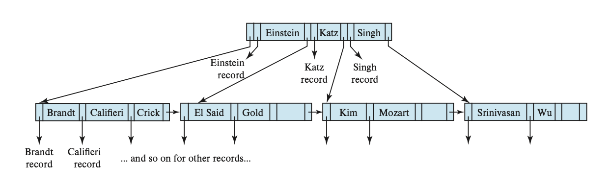
When searching on a B-tree, we may sometimes find the desired value before reaching the leaf nodes. However, since non-leaf nodes contain fewer search keys compared to B+ trees—meaning they have a lower fan-out—a B-tree is taller than a B+ tree storing the same content. In general, the search time on a B-tree is proportional to the logarithm of the number of search keys.

The deletion operation in a B-tree is more complex because the deleted item may also appear in non-leaf nodes. Specifically, if a search key $K_i$ is deleted, the smallest search key in the subtree pointed to by $P_{i+1}$ must be moved to the position originally occupied by $K_i$ .

For larger-scale indexes, the space advantage of B-trees is not significant. Therefore, most database systems still use B+ trees.

Indexing on Flash Storage

In the previous introduction, we assumed that data is stored on a hard disk. Now, let’s look at the case of using indexes for flash memory or SSDs.

The node size of the B+ tree matches the page size of the flash memory.
The bottom-up construction method also reduces page write operations.
To reduce the number of erasures on flash memory, one approach is to add a buffer to the internal nodes of the B+ tree to temporarily record updates, and then propagate the update operations down to lower-level nodes. Another approach is to create multiple trees and merge them.

Indexing in Main Memory

Of course, data in memory can also be indexed.

If the nodes of a B+ tree are small enough to fit in a cache line, it will bring better performance for in-memory data, because such a B+ tree can reduce the number of cache misses encountered during index operations.

10.4 Hash Indices

Hashing indexes may be temporarily used for join operations or as permanent structures in main-memory databases.

The average time complexity of accessing a hash table is $O(1)$ (the worst-case time complexity is $O(n)$ , and the space complexity is $O(1)$ , but in practice, we cannot ignore the impact of constants.

The implementation of a hash table includes the following components:

Hash functions: These map a large key space into a smaller domain, used to compute the index position of an array (bucket or slot).
Hash schemes: Methods for handling collisions after hashing. We need to balance between reducing collisions by allocating a larger hash table and performing additional operations when collisions occur.

In hashing, a bucket refers to a storage unit that holds one or more records, typically a linked list of index entries or records (used in hash file organization).

Overflow chaining: To insert a record with a search key value $K_i$ , we first compute $h(K_i)$ to obtain the bucket address for that record, then add the index entry of this record to the list at offset $i$ .

Hash indexes support equality queries on search keys (just compare hash function values) but do not support range queries (whereas B+ trees support both). Deletion operations are straightforward: after using the hash function to locate the corresponding bucket, simply delete the specified record from the bucket.

For insertion operations, if the bucket does not have enough space, a bucket overflow occurs, and overflow buckets are used to resolve this issue.

If a record must be inserted into bucket $b$ , and $b$ is full, the system will provide an overflow bucket for $b$ and insert the record into this overflow bucket. If the overflow bucket is also full, the system will provide another overflow bucket, and so on. These overflow buckets are linked together using a linked list, forming the previously mentioned overflow chain.

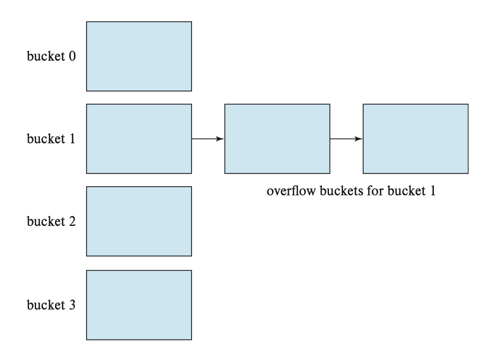
If we can know the number of records to be indexed in advance, we can allocate sufficiently large buckets, thereby avoiding the problem of bucket overflow.

When multiple records have equal search key values, it leads to an uneven distribution (or skew) of records across all buckets, which is likely due to a poorly chosen hash function.

To reduce the probability of bucket overflow, we set the number of buckets to $\dfrac{n_r}{f_r} \cdot (1 + d)$ , where $n_r$ is the total number of records, $f_r$ is the number of records per bucket, and $d$ is an arbitrary value (fudge factor), typically set to around 0.2. In this case, 20% of the space in the bucket is empty. Although this may seem like a waste of space, it helps reduce the occurrence of bucket overflow.

The hash indexes introduced earlier all have a fixed number of buckets, a method known as static hashing. It has a problem: we need to know how many records are stored in the index; otherwise, the bucket capacity may be insufficient.

To address this issue, when the number of records reaches a certain level, the hash index must be reconstructed to increase the number of buckets, but this process can be time-consuming. Hash indexes that allow the number of buckets to grow are called dynamic hashing, and both linear hashing and extendable hashing fall into this category.

10.5 Multiple-Key Access

composite search keys: A search key composed of multiple attributes. In this case, the order of the search key values follows lexicographic ordering.

However, this type of search key is not suitable for queries where both attributes are range conditions, for example:

SELECT ID
FROM instructor
WHERE dept_name < 'Finance' AND salary < 80000;

Because these records that meet the condition may be located in different disk blocks, and the records within the file are ordered, this will result in a large number of I/O operations.

covering indices: An index that stores certain attributes (not search key attributes) along with pointers to records. Using this type of index can reduce the size of search keys, thereby allowing for greater deletion in non-leaf nodes and lowering the height of the index tree.

10.6 Indices in SQL

Most databases support creating and deleting indexes using SQL commands, with the syntax format roughly as follows:

CREATE INDEX <index-name> ON <relation-name> (<attribute-list>);
DROP INDEX <index-name>;

If you want to use a candidate key as a search key, you can achieve this with CREATE UNIQUE INDEX.

When a user’s query can benefit from an index, the SQL query processor will automatically use that index.

However, creating too many indexes can slow down update processing, because update operations also affect all impacted indexes. Therefore, before creating an index, you should first consider whether it is truly necessary.

If a relation has a primary key, most database systems will automatically create an index based on it. If this is not done, the entire relation would need to be scanned when inserting tuples to ensure that the primary key constraint is satisfied.

10.7 Write-Optimized Index Structure

Some write-optimized index structures to handle the workload caused by high write/insert rates.

LSM Trees

LSM tree, short for log-structured merge tree, is composed of multiple B+ trees, including an in-memory tree $L_0$ and trees on disk $L_1, L_2, \dots, L_k$ , where $k$ is referred to as the level.

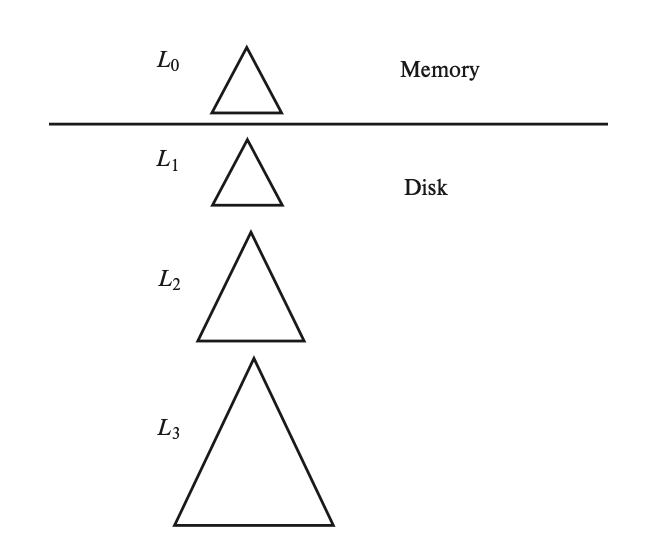
The search process of the index is as follows: first, perform a separate search operation on each tree, and then merge the search results.

When inserting a record into the LSM tree,

First, insert the record into $L_0$ in memory (the system allocates a considerable amount of memory space for it). If the memory space is full, the data must be moved from memory to the B+ tree on the hard disk.
Specifically, if $L_1$ is empty, then the entire $L_0$ is written to $L_1$ ; otherwise, scan the leaf level of $L_0$ in ascending order of keys, and then merge the items in it with the items in the leaf level of $L_1$ (also requiring scanning). Then, using a bottom-up construction method, create a new B+ tree based on the merged items, and replace the old $L_1$ with this new tree.

However, copying a tree incurs significant costs, so here are some methods to reduce costs:

Use a multi-level tree, where the maximum capacity of tree $L_{i+1}$ is $k$ times that of $L_i$ , so each record is written at most $k$ times. The number of levels is proportional to $\log_k (I/M)$ , where $I$ is the total number of items and $M$ is the number of items in $L_0$ .
Except for $L_0$ , each level has at most $b$ trees (originally only 1 tree). This variant is called a stepped-merge index, which significantly reduces insertion costs but increases query costs.

The deletion operation does not require deleting existing index entries; instead, a deletion entry is inserted to indicate which index entry has been deleted. The process of inserting a deletion entry is the same as inserting a normal index entry. Therefore, the search operation requires an additional step: if some entries have deletion entries, then when searching for a specified search key, both the original index entry and the deletion entry need to be found. If a deletion entry is found, the original index entry is not returned.

The update operation is similar to deletion, requiring the insertion of an update entry. The update is completed during the merge operation.

Buffer Trees

A buffer tree is built upon the B+ tree, where each internal node (including the root node) has an associated buffer. The structure of a node is as follows:

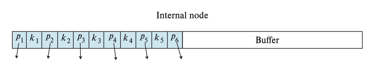
Insertion:

When inserting an index record, instead of traversing leaf nodes first, it is first inserted into the buffer of the root node. All records in the buffer are sorted by their search keys.
If the buffer is full, each index record in the buffer is pushed down to the buffer of the appropriate child node at the next level, and so on.
If the next-level node is a leaf node, the index record is inserted into the leaf node using the normal method.
If the leaf node is full, a split operation is performed. This may cause internal nodes to split as well, and the corresponding buffers also need to be split.

Search:

Compared to a standard B+ tree search, there is an additional step: when traversing internal nodes, check whether the search key exists in the node’s buffer.

Deletion and Update:

Similar to LSM trees, deletion entries and update entries need to be inserted.
Standard B+ tree algorithms can also be used, but this results in higher I/O costs.

In the worst case, the upper bound on the number of I/O operations for a buffer tree is lower than that of an LSM tree. For read operations, the buffer tree is significantly faster than the LSM tree. However, for write operations, the buffer tree performs worse because it requires more random I/O, leading to higher seek time.

Therefore, when write operations are more frequent, the LSM tree is preferred; when read operations are more frequent, the buffer tree is preferred.

B $\varepsilon$ -Trees

We do not immediately update the B+ tree; instead, we store the updates in the log cache of the corresponding key-value entries in the internal nodes. Such a tree is called a fractal tree or $B\varepsilon$ tree. When the buffer is full, updates are incrementally propagated downward to lower-level nodes.

10.8 Bitmap Indices

Bitmap indices are a type of index suitable for simple queries on multiple keys.

Before using bitmap indices, each record in the relation needs to be labeled (starting from 0). This operation is straightforward if the records are of fixed size and allocated in consecutive blocks within a file, as the record number can then be converted into a block number.

A bitmap is a set of bits. For an attribute $A$ of a relation $r$ , the bitmap index contains each possible value of $A$ , and the number of bits corresponds to the number of records. For a bitmap of a specific value $v_j$ , if the attribute value of the record numbered $i$ is $v_j$ , then the $i$ -th bit of that bitmap is set to 1; otherwise, it is set to 0.

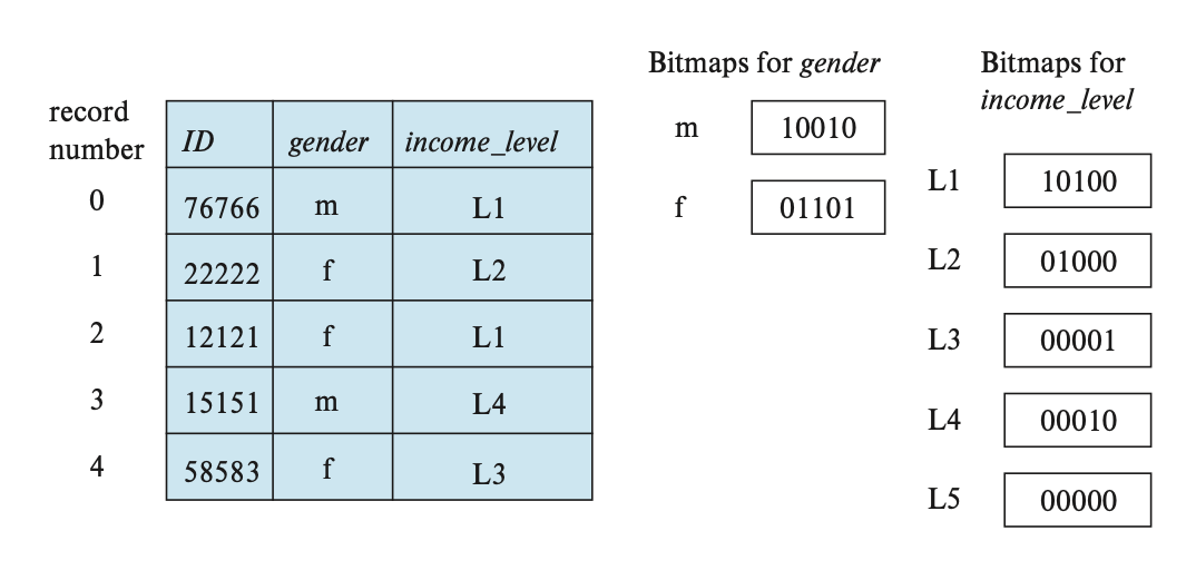
For the following query:

SELECT *
FROM instructor_info
WHERE gender = 'f' AND income_level = 'L2';

We find the bitmap where the $gender$ attribute value is f and the $income\_level$ attribute value is L2, and then perform an intersection operation (which is essentially a logical AND operation) on these two bitmaps. The record with ID 1 is the record we want to query.

Chapter 11 Query Processing

parsing & translation
- The parser translates the query statement into an internal form that the system can understand.
- The system constructs a parse tree for the query, which is then translated into a relational algebra expression.
- If the query is expressed in the form of a view, all views are translated into relational algebra expressions that define the view.
optimization
- The system is responsible for generating a query evaluation plan that minimizes the cost of query evaluation.
evaluation
- Provides relational algebra expressions.
- Annotates them with instructions indicating how to perform the evaluation operations.
- The query-execution engine is responsible for generating and executing the query evaluation plan, as well as returning the query results.

evaluation primitive: A relational algebra operation annotated with instructions.
query-execution/evaluation plan: A sequence composed of these primitives.

The following diagram illustrates the complete query processing flow:

11.1 Measures of Query Costs

The cost of query evaluation includes disk access, CPU time for executing the query, and communication time in parallel or distributed database systems.

For large databases, I/O cost is the most significant; for databases stored in memory or on SSDs, the main cost is CPU cost.

When estimating the cost of a query evaluation plan, we measure it using two factors: the number of block transfers and the number of random I/O accesses (corresponding to disk seek times).

We use $t_T, t_S$ to denote the average time to transfer one data block and the average block access time (disk seek time + rotational latency), respectively. Therefore, if an operation requires transferring $b$ data blocks and $S$ random I/O accesses, the time required is $b \cdot t_T + S \cdot t_S$ .

Although SSDs do not involve seek time, they still require some time to initiate I/O operations. Thus, we set $t_S$ as the time from initiating an I/O request to the return of the first byte of data.

The cost of an algorithm depends on the size of the main memory buffer. In the best case, the buffer can hold all the data, eliminating the need for further disk accesses; in the worst case, the buffer can only hold a portion of the data blocks.

For B+ tree indexes, most database systems assume that all internal nodes are in the memory buffer and that a single traversal of the index requires only one random I/O cost for accessing a leaf node.

The response time of a query evaluation plan—the time required to execute the plan—is difficult to estimate.

11.2 Selection Operations

Selections Using File Scans and Indices

File scans are the lowest-level operations for accessing data, serving as search algorithms that locate and retrieve records meeting selection conditions.

The simplest algorithm is linear search (labeled A1): the system scans each file block, examining all records to determine if they satisfy the selection condition.

Accessing the first block of a file requires an initial seek; additional seeks are needed for non-contiguous blocks, but we ignore this effect here.

This algorithm works for any file; other algorithms, while not applicable in all cases, are always faster than linear search when they are applicable.

The figure below shows linear search and the estimated costs of some algorithms introduced later.

Various Sequential Scan Optimization Techniques
Compression: Allows retrieving more tuples in a single fetch, e.g., RLE.
Prefetching: Fetches some pages in advance so the DBMS does not need to block on storage I/O operations when accessing each page.
Buffer Pool Bypass: The scan operator stores pages fetched from disk directly in local memory instead of the buffer pool, avoiding the “sequential flooding” problem.
Parallelization: Uses parallel multi-threading/processes to execute scan operations.
Late Materialization: DSM (Decomposition Storage Model) DBMS can delay tuple assembly until later stages of the query plan. This design allows each operator to pass only the minimal necessary information (e.g., record IDs, offsets of records in columns) to the next operator. This feature is only practically useful in columnar storage systems.
Heap Clustering: Tuples are stored in heap pages in the order specified by a clustered index.
Result Caching/Materialized View: Stores results of frequently occurring subqueries/queries.
Code Specification/Compilation: Pre-compiles functions in advance to retrieve results faster when needed.
Approximate Queries (Lossy Data Skipping): Executes queries on a sampled subset of the entire table to generate approximate results, often used for computing aggregate data with a margin of error to obtain near-accurate answers.
Zone Maps (Lossless Data Skipping): Precomputes aggregate values for each tuple attribute in a page, allowing the DBMS to decide whether to access a page by first checking its zone map.

Search algorithms using indexes are called index scans. This category includes:

A2 (Clustered Index, Equality Condition on Key): Uses the index to retrieve a single record satisfying the corresponding equality condition.
A3 (Clustered Index, Equality Condition on Non-Key Attribute): Differs from the previous case in that multiple records need to be retrieved, and these records must be stored contiguously in the file because the file is sorted by the search key.
A4 (Secondary Index, Equality Condition):
- Equality Condition on Key: Similar to A2.
- Equality Condition on Non-Key Attribute: Each record may be located in a different block, requiring one I/O operation per record retrieved, which includes one seek and one block transfer. In the worst case, the cost is $(h_i + n) \cdot (t_S + t_T)$ , where $n$ is the number of records retrieved, $h_i$ is the height of the B+ tree, assuming each record is on a different disk block and these blocks are randomly ordered.

For the above algorithms, if a B+ tree file organization is used, one access can be saved because all records are stored at the leaf level of the tree. In this case, the secondary index stores attribute values that serve as the search key for the B+ tree file organization rather than direct pointers to records, but this makes record access more costly.

Selections Involving Comparisons

The following algorithm can handle selections of the form $\sigma_{A \le v}(r)$ :

A5 (clustered index, comparison condition)
- For comparisons of the form $A > v$ or $A \ge v$ , first locate the index of $v$ to find the first tuple that satisfies the condition; then perform a file scan starting from that tuple until the end of the file.
- For comparisons of the form $A < v$ or $A \le v$ , there is no need to first perform an index lookup. Instead, start a file scan from the beginning of the file until the first index that satisfies $A = v$ or $A > v$ is found. In this case, the index is not particularly useful.
A6 (secondary index, comparison condition): As mentioned earlier, the cost of accessing a single record using this method is too high, so it is rarely used unless very few records are selected.

If the number of matching tuples can be known in advance, the query optimizer can choose between using a secondary index or a linear scan based on cost estimation. However, when the exact number cannot be determined at compile time, PostgreSQL employs a hybrid algorithm called bitmap index scan.

Implementation of Complex Selections

Now let’s consider more complex selection predicates:

Conjunction: $\sigma_{\theta_1 \wedge \theta_2 \wedge \dots \wedge \theta_n}(r)$
Disjunction: $\sigma_{\theta_1 \vee \theta_2 \vee \dots \vee \theta_n}(r)$
Negation: $\sigma_{\neg \theta}(r)$
A7 (Conjunctive selection using a single index): First, determine whether there is an access path (i.e., a corresponding index structure) for a certain attribute under a simple condition. If so, use the algorithms from A2-A6 to retrieve the records that satisfy the condition. Then, in the memory buffer, check whether the retrieved records satisfy the remaining simple conditions to complete the entire operation. To minimize cost, for each simple condition $\theta_i$ , we select the algorithm with the lowest cost for $\sigma_{\theta_i}(r)$ from A1-A6.
A8 (Conjunctive selection using a composite index): If the selection condition involves equality comparisons on multiple attributes and there is a composite index composed of these attributes, the index can be directly searched. In this case, we use the algorithms from A2-A4.
A9 (Conjunctive selection using intersection of identifiers): The intersection of all record identifiers (or record pointers) yields a set of pointers to tuples that satisfy the conjunctive condition. The cost of this algorithm includes separate index scans and the cost of retrieving records. The cost can be reduced by sorting the pointers.
A10 (Disjunctive selection using union of identifiers): Similar to A9.

11.3 Sorting

We can sort relationships by building an index based on search keys and then reading the relationships according to the index. However, this only sorts the relationships at a logical level, whereas we aim to sort them at a physical level.

External Sort-Merge Algorithm

When the main memory cannot hold all the data, the sorting algorithm we use is called external sorting, and one of the most commonly used external sorting techniques is the external sort-merge algorithm.

Let $M$ be the number of blocks in the main memory buffer available for sorting. The execution steps of this sorting process are as follows:

Create a set of sorted runs. Each run is internally sorted but contains only a portion of the records from the relation. For sorted runs, we have two strategies: early materialization (storing the entire tuple within a page) and late materialization (storing only the record ID within a page).
Merge these runs. For now, we assume that the total number of runs $N < M$ , so we can allocate one block for each run and have remaining space for storing the output data block.

The output of the merge phase is a sorted relation. The output file needs to be buffered to reduce the number of disk write operations. This merge operation is essentially a generalization of the two-way merge used in standard in-memory merge sort algorithms. If we are merging $N$ runs, this operation is called an N-way merge.

However, in general, if the size of the relation exceeds the memory capacity, the first step may produce no fewer than $M$ runs. Consequently, during the merge process, it may not be possible to allocate a memory block for each run. In this case, the merge operation needs to be carried out in multiple passes, with each pass merging at most $M-1$ runs as input.

The process of the first pass is as follows: merge the first $M-1$ runs to produce a new run for the next pass; then merge the next $M-1$ runs, and so on, until all initial runs have been processed.

At this point, the number of runs is reduced to $\dfrac{1}{M-1}$ of the original. If this number is still no less than $M$ , another pass is needed, and this process repeats until the number of passes is less than $M$ . The result of the final pass is the ultimately sorted output.

Example: Calculating the number of passes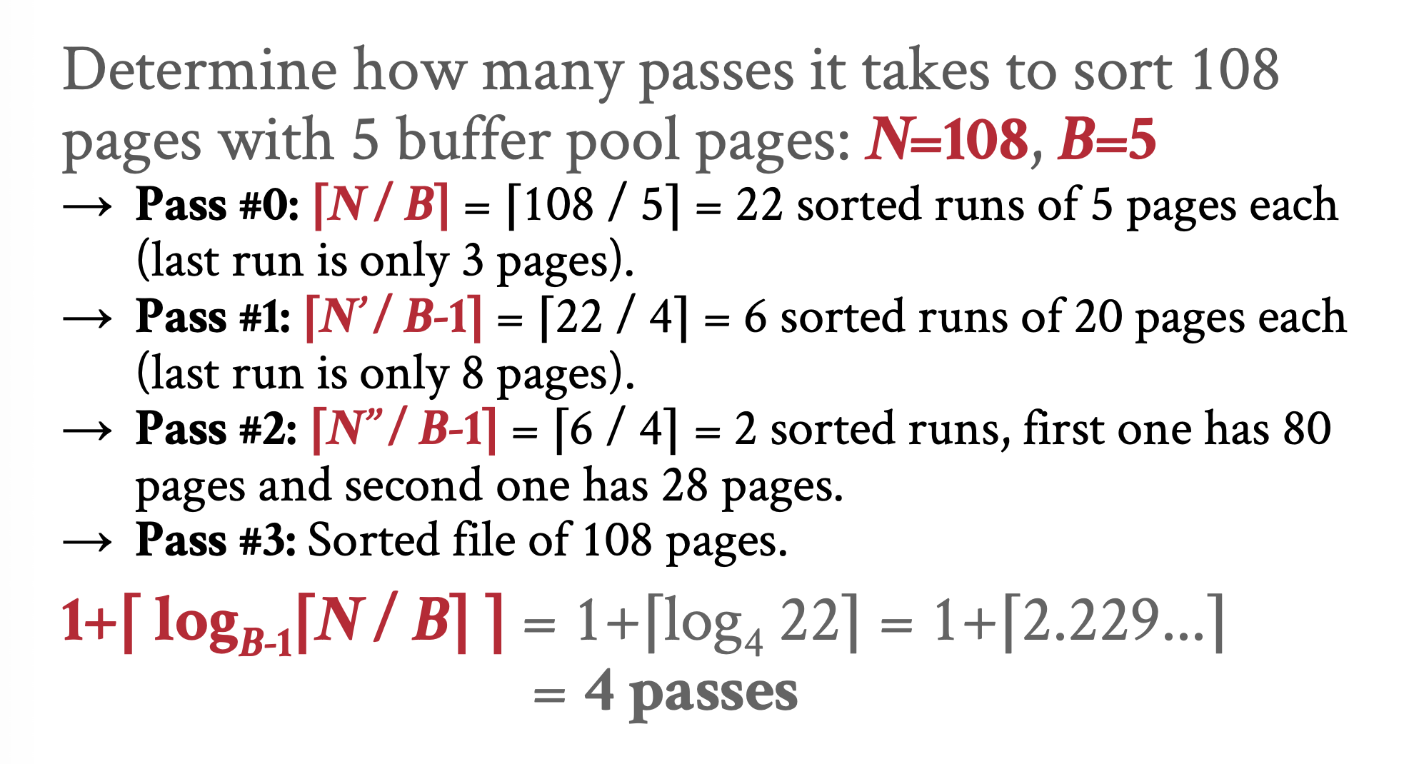

Cost Analysis

Disk Access Cost:

Let $b_r$ be the number of blocks containing the tuples of relation $r$ . In the first phase, each block requires one read and one write operation, resulting in a total of $2b_r$ block transfers.
The initial number of runs is $\lceil \dfrac{b_r}{M} \rceil$ .
During merging, reading one run from a data block at a time incurs a large number of seek operations. To reduce the number of seeks, we allocate $b_b$ larger buffer blocks for each input run and output run. Therefore, each pass can merge $\lfloor \dfrac{M}{b_b} - 1 \rfloor$ runs, meaning the number of runs after each merge is reduced to $\frac{1}{\lfloor \dfrac{M}{b_b} - 1 \rfloor}$ of the original.
The total number of merge passes is $\lceil \log_{\lfloor \frac{M}{b_b} - 1 \rfloor} (\dfrac{b_r}{M}) \rceil$ .
Each pass involves one read and one write operation for every data block, except in the following two cases: the output from the last pass does not need to be written to disk; some runs may neither be read nor written in a certain pass. Here, we ignore this special case.
The total number of block transfers is: $b_r(2\text{pass}+1)=b_r(2\lceil \log_{\lfloor \frac{M}{b_b} - 1 \rfloor} (\dfrac{b_r}{M}) \rceil + 1)$ .

Disk Seek Cost:

During run generation, read and write operations are required for each pass.
Each merge pass requires approximately $\lceil \dfrac{b_r}{b_b} \rceil$ seeks for reading and writing data, respectively, totaling $2 \lceil \dfrac{b_r}{b_b} \rceil$ seeks (except for the last pass).
The total number of seeks is: $2 \lceil \dfrac{b_r}{M} \rceil + \lceil \dfrac{b_r}{b_b} \rceil (2 \text{pass} - 1) = 2 \lceil \dfrac{b_r}{M} \rceil + \lceil \dfrac{b_r}{b_b} \rceil (2\lceil \log_{\lfloor \frac{M}{b_b} - 1 \rfloor} (\dfrac{b_r}{M}) \rceil - 1)$ .

Optimization of Comparison Operations

Code Specialization: Instead of providing a comparison function as a pointer to the sorting algorithm, create a hardcoded sorting version specific to a particular key type.

Suffix Truncation: First compare the binary prefix of long VARCHAR keys, rather than slower string comparison; if the prefixes are the same, fall back to the slower comparison method.

11.4 Join Operations

Now let’s learn about some algorithms used to compute relational connections and analyze the costs of these algorithms.

Nested-Loop Join

The relation $r$ is called the outer relation, and $s$ is called the inner relation.

This algorithm does not require the use of indexes and is applicable to any join condition.

The cost of this algorithm is relatively high because it needs to examine every pair of tuples from the two relations.

In the worst case, the buffer can only hold one block for each relation, thus requiring $n_r \cdot b_s + b_r$ block transfers (where $n_r, n_s$ represent the number of tuples in $r, s$ respectively, and $b_r, b_s$ represent the number of blocks containing tuples of $r, s$ respectively) and $n_r + b_r$ seeks.

In the best case, the memory can hold both relations simultaneously, thus requiring only $b_r + b_s$ block transfers and 2 seeks.

If the memory can only hold one complete relation, it is best to place the inner relation $s$ in memory, because then the inner relation only needs to be read once. The cost in this case is the same as in the best-case scenario.

Block Nested-Loop Join

If the buffer is too small to hold any complete relation, we can reduce the number of block accesses by reading the relation in blocks rather than by tuples.

In the worst case, for each block of the outer relation, only one block of the inner relation can be read, requiring $b_r \cdot b_s + b_r$ block transfers and $2 \cdot b_r$ seeks. It is easy to see that using the smaller relation as the outer relation makes the operation more efficient.

In the best case, when the inner relation can fit in memory, only $b_r + b_s$ block transfers and 2 seeks are needed.

The performance of nested-loop and block nested-loop joins can be further improved through the following methods:

If the join attributes in a natural join or equi-join form a key of the inner relation, then for each tuple of the outer relation, the inner loop can terminate immediately upon finding the first matching tuple.
In block nested-loop joins, we use the largest block that memory can accommodate (while reserving enough space for the inner relation and output). In other words, assuming there are $M$ memory blocks, we read $M - 2$ blocks from the outer relation each time (with the remaining two blocks, one for input and one for output). This reduces the number of scans of the inner relation from $b_r$ to $\lceil \dfrac{b_r}{M-2} \rceil$ , and the cost becomes $\lceil \dfrac{b_r}{M-2} \rceil \cdot b_s + b_r$ block transfers and $2 \lceil \dfrac{b_r}{M-2} \rceil$ seeks.
We can alternately scan the loops forward and backward, sorting the disk blocks so that data remaining in the buffer can be reused, thereby reducing disk access times.
If an index on the join attribute of the inner loop is available, file scans can be replaced with more efficient index lookups. This method is introduced below.

Indexed Nested-Loop Join

The cost of this method is:

For each tuple in the outer relation $r$ , a lookup is performed on the index of $s$ , and the relevant tuples are retrieved.
In the worst case, the buffer space can only accommodate one block of $r$ and one block of the index. Therefore, reading $r$ requires $b_r$ I/O operations (including one seek and one block transfer). Thus, the cost of the join at this point is $b_r(t_T + t_S) + n_r \cdot c$ , where $c$ is the cost of performing a single selection on $s$ using the join condition.

Merge Join

Algorithm

The algorithm requires that the tuples in $S_s$ fit into main memory. If the size of $S_s$ exceeds the available memory, a block nested loop join can be used, matching two blocks from $r$ and $s$ with the same join attribute values.

If the input relations $r$ and $s$ are not sorted based on the join attribute, they need to be sorted first (using the algorithm introduced in the previous section).

Cost Analysis

Once the relationship is sorted (here referring to the physical level), the tuples with the same join attribute values are consecutive in order. Therefore, each tuple only needs to be read once, and each block only needs to be read once as well. The number of block transfers is $b_r + b_s$ .

Assuming $b_b$ buffer blocks are allocated for each relationship, the number of disk seeks is $\lceil \dfrac{b_r}{b_b} \rceil + \lceil \dfrac{b_s}{b_b} \rceil$ . Since seeks are more costly than block transfers, we should allocate as many buffer blocks as possible for each relationship.

If the input relationships $r, s$ are not yet sorted, we also need to consider the cost of sorting. Additionally, if the memory cannot fully accommodate $S_s$ , there will be an additional small cost.

Hybrid Merge Join

If there is a secondary index on the join attribute, we can execute a variant of the merge join on unsorted tuples. This algorithm scans records through the index, and the retrieval order is sorted. However, this method has a significant drawback: since records may be scattered across different disk blocks, each tuple access results in a disk block access, making the cost quite high.

To avoid this cost, we adopt a technique called hybrid merge-join, which combines indexing and merge join. Based on the above assumption (and assuming the secondary index uses a B+ tree), we merge the sorted relation according to the leaf entries of the secondary B+ tree index. The resulting file contains tuples from the sorted relation along with the addresses of those tuples in the unsorted relation. This result file is then sorted by these addresses, allowing efficient retrieval of the corresponding tuples in physical storage order, thereby completing the join operation.

Hash Join

We use a hash function $h$ to partition the tuples in the two relations, specifically by placing tuples with the same hash value on the join attributes into the same partition. We assume:

$h$ is a hash function that maps $JoinAttrs$ values to $\{0, 1, \dots, n_h\}$ , where $JoinAttrs$ are the common attributes of $r$ and $s$ in the natural join.
The partitions $r_0, r_1, \dots, r_{n_h}$ represent the partitioning of tuples from $r$ , each initially empty, and each tuple $t_r \in r$ is placed in partition $r_i$ , where $i = h(t_r[JoinAttrs])$ .
The partitions $s_0, s_1, \dots, s_{n_h}$ represent the partitioning of tuples from $s$ , each initially empty, and each tuple $t_s \in s$ is placed in partition $s_i$ , where $i = h(t_s[JoinAttrs])$ .

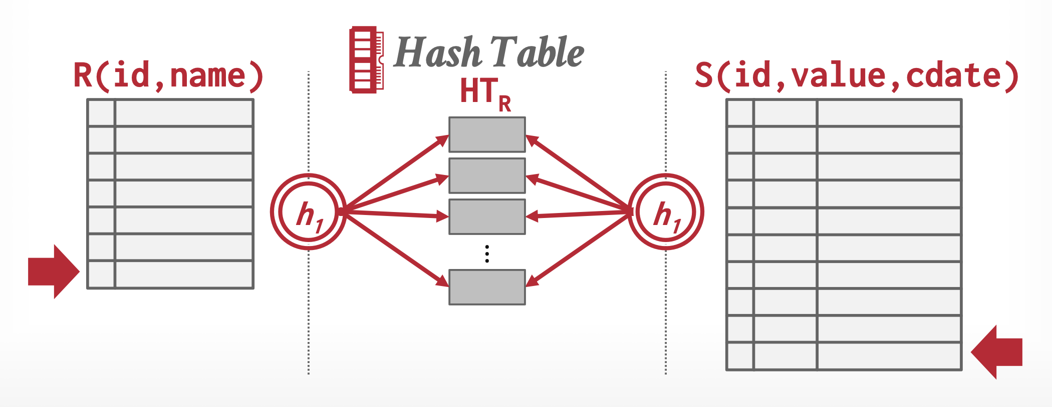
Basics

The basic idea of hash join is: suppose a tuple from $r$ and a tuple from $s$ satisfy the join condition, meaning they have the same join attribute value. If this value is mapped to value $i$ by a hash function, then the tuple from $r$ is placed into partition $r_i$ , and the tuple from $s$ is placed into partition $s_i$ . Therefore, tuples in $r_i$ only need to be compared with tuples in $s_i$ , without considering tuples in other partitions.

After partitioning the relationship, a separate index nested loop join must be performed for each partition $i\ (i = 0, \dots, n_h)$ . Specifically,

First, a hash index is built for each $s_i$ :
Then, the corresponding tuples are probed (i.e., looked up) from $r_i$ :

Thus, the relations $s, r$ are called the build input and probe input, respectively.

The hash index for $s_i$ is built in memory, so there is no need to access tuples from disk. Note that the hash function used for building the hash index must be different from the one used for partitioning, but it still operates only on the join attributes. In an index nested loop join, the system uses the hash index to retrieve records that match the records in the probe input.

Here, the size of $n$ must be large enough so that for each $i$ , the tuples of the build relation partition $s_i$ and its hash index can fit in memory. However, it is not necessary for the probe relation partition to be fully contained in memory. Therefore, the smaller relation is chosen as the build relation.

If the build relation contains $b_s$ blocks, and each partition does not exceed $M$ in size, then the number of partitions $n_h$ must be at least $\lceil \dfrac{b_s}{M} \rceil$ .

However, if the memory size (assuming it can hold at most $M$ data blocks) is insufficient, then the number of partitions is at most $M - 1$ (with one block reserved as an input buffer).

Recursive Partitioning

If $\lceil \dfrac{b_s}{M} \rceil$ is greater than $M - 1$ , the relation cannot be fully partitioned in a single pass because there are not enough buffer blocks.

Therefore, the partitioning process must be completed over multiple passes—in each pass, as many partitions as possible are created while reserving enough buffer space for output. Each bucket obtained from a pass is read and partitioned separately in the next pass to create smaller partitions.

Note that the hash function used in each pass is different. The system will repeat the partitioning operation until each partition of the build input can fit into memory.

When $M > n_h + 1$ , i.e., $M > \dfrac{b_s}{M} + 1$ (which can be simplified (approximately) to $M > \sqrt{b_s}$ ), the relation does not require recursive partitioning.

Assuming the table r and s has 256 and 1024 blocks respectively. Each block has 4K bytes. To do natural join r and s with the Hash Join algorithm, what is the approximate minimum memory needed to avoid recursive partitioning?
取较小的那个关系 $S$ 作为构建关系，块数 $b_s = 256$ ，所以 $M_{\min} = 4KB \times \sqrt{256} = 64KB$

$M ≥ \sqrt{b_{build}}$

Handling of Overflows

In constructing the partition $i$ of the build relation $s$ , if the hash index size of $s_i$ exceeds the memory capacity, a hash-table overflow problem occurs.

The underlying cause of this issue may be that many tuples in the build relation have the same join attribute value, or the hash function lacks good randomness and uniformity, leading to some partitions containing more than the average number of tuples while others contain fewer—such partitions are considered skewed.

To handle minor skew, we can increase the number of partitions so that each partition’s size is smaller than the memory capacity. The additional amount is called the fudge factor, typically around 20%.

However, even this may not always resolve the overflow issue. In such cases, the following methods can be used:

Overflow resolution: If an overflow is detected during the build phase, the corresponding partition (applicable to both $s_i$ and $r_i$ ) is repartitioned using a different hash function into smaller partitions.

Overflow avoidance: Carefully execute the partitioning operation to prevent overflow during the build phase. Specifically, initially partition the build relation $s$ into many small partitions, then combine some partitions that together fit into memory. The probe relation can be handled similarly.

Nevertheless, these two methods may still fail in more extreme cases. In such situations, we can try other join techniques, such as block nested loop join.

Cost Analysis

If recursive partitioning is not used,

Partitioning the two relations $r, s$ requires one read and one write operation, totaling $2(b_r + b_s)$ block transfers. The build and probe phases require reading each partition once, thus needing an additional $b_r + b_s$ block transfers. The number of blocks occupied by the partitions may be slightly more than $b_r + b_s$ , resulting in some blocks that are only partially filled. For each relation, accessing such blocks incurs at most $2n_h$ overhead. Therefore, the total block transfers are $3(b_r + b_s) + 4n_h$ , where $4n_h$ is usually much smaller than the previous term and can be ignored.
If $b_b$ blocks are allocated for input and output buffers, partitioning requires $2(\lceil \dfrac{b_r}{b_b} \rceil + \lceil \dfrac{b_s}{b_b} \rceil)$ seeks. In the build and probe phases, for the $n_h$ partitions of each relation, only one seek is needed each. Thus, the total number of seeks is $2(\lceil \dfrac{b_r}{b_b} \rceil + \lceil \dfrac{b_s}{b_b} \rceil) + 2n_h$ .

If recursive partitioning is used,

Each partitioning pass reduces the number of partitions to $\lceil \dfrac{M}{b_b} - 1 \rceil$ of the original, and the expected number of passes is $\lceil \log_{\lfloor \frac{M}{b_b} - 1 \rfloor}\dfrac{b_s}{M} \rceil$ .
In each pass, every block of $s$ is read and written once, so the number of block transfers when partitioning $s$ is $2b_s \lceil \log_{\lfloor \frac{M}{b_b} - 1 \rfloor}\dfrac{b_s}{M} \rceil$ . The number of block transfers required when partitioning $r$ is essentially the same as when partitioning $s$ , so the total number of block transfers is: $2(b_r + b_s) \lceil \log_{\lfloor \frac{M}{b_b} - 1 \rfloor}\dfrac{b_s}{M} \rceil + b_r + b_s$ .
Ignoring the few seeks needed in the build and probe phases, the total number of seeks is $2(\lceil \dfrac{b_r}{b_b} \rceil + \lceil \dfrac{b_s}{b_b} \rceil) \lceil \log_{\lfloor \frac{M}{b_b} - 1 \rfloor}\dfrac{b_s}{M} \rceil$ .

If the main memory is large enough to hold the entire build input, then $n_h = 0$ , and no partitioning of the relations is needed. In this case, only $b_r + b_s$ block transfers and 2 seeks are required.

Complex Joins

Let us consider join operations with more complex join conditions—conditions that include conjunctions and disjunctions. We can combine some of the previously introduced algorithms for complex selections with join techniques to handle such cases.

For joins with conjunction conditions: $r \bowtie_{\theta_1 \wedge \theta_2 \wedge \dots \wedge \theta_n} s$ , we can first compute the join under one simple condition $r \bowtie_{\theta_i} s$ , and then check whether the tuples in this intermediate result satisfy the remaining conditions $\theta_1 \wedge \dots \wedge \theta_{i-1} \wedge \theta_{i+1} \wedge \dots \wedge \theta_n$ .
For joins with disjunction conditions: $r \bowtie_{\theta_1 \vee \theta_2 \vee \dots \vee \theta_n} s$ , the computation can be completed by taking the union of the records from individual joins $r \bowtie_{\theta_i} s$ : $(r \bowtie_{\theta_1} s) \cup (r \bowtie_{\theta_2} s) \cup \dots \cup (r \bowtie_{\theta_n} s)$ .

Summary: Comparing the costs of various join algorithms

Among them, $M, N$ represent the number of data blocks for relations $R, S$ respectively, $m, n$ represent the number of tuples for relations $R, S$ respectively, and $C$ represents a constant. The I/O cost here corresponds to the number of data transfers.

11.5 Other Operations

Duplicate Elimination

We can first sort the relation. After sorting, identical tuples will appear in adjacent positions, but only one copy is retained.

In the external sort-merge algorithm, we can detect and remove duplicates when creating runs, before writing them to disk, thereby reducing the number of block transfers. The remaining duplicates can be eliminated during the merge phase, so that the final sorted runs contain no duplicates. Thus, in the worst case, the cost of eliminating duplicates is the same as the cost of sorting the relation.
In the hash join algorithm, we can also use hashing to remove duplicates. When building a hash index for each partition, we only insert tuples that do not already exist; otherwise, we discard the tuple. After all tuples in a partition have been processed, its hash index is written to the result. Therefore, the cost of deduplication in this case is the same as the cost of processing the build relation.

Projection

Performing a (generalized) projection operation on the entire relation requires projecting each tuple. This can easily result in duplicate entries, which need to be removed. The method for doing so is described above.

Set Operations

Set operations include union, intersection, and difference. For these operations, only one scan of the two sorted relations is required, so the number of block transfers is $b_r + b_s$ . If the relations are not sorted, the cost of sorting must also be considered.

In the worst case, if each relation has only one block buffer, then $b_r + b_s$ seeks are also required. Therefore, the number of seeks can be reduced by allocating additional buffer blocks.

Hash-based implementation can also be used for set operations: first partition the two relations separately using the same hash function, and then handle each case as follows:

$r \cup s$ $r \cup s$
- Build an in-memory hash index for $r_i$
- When a tuple from $s_i$ does not appear, add it to the hash index
- Add the tuples from the hash index to the result
$r \cap s$ $r \cap s$
- Build an in-memory hash index for $s_i$
- For each tuple in $s_i$ , probe the hash index; if the tuple appears in the hash index, output it
$r - s$ $r - s$
- Build an in-memory hash index for $r_i$
- When a tuple from $s_i$ appears in the hash index, delete it from the hash index
- Add the tuples from the hash index to the result

Outer Join

There are two methods to implement outer join operations:

First compute $r \bowtie s$ , then add the tuples that additionally appear in $r$ ⟕ $_\theta s$ and $r$ ⟖ $_\theta s$ , thus forming the complete $r$ ⟗ $_\theta s$ .
- To compute $r$ ⟕ $_\theta s$ , first compute $r \bowtie_\theta s$ and temporarily store the result in relation $q_1$ ; then compute $r - \Pi_R(q_1)$ to obtain those tuples of $r$ that did not participate in the theta join, fill these tuples with null values, and add them to $q_1$ to get the final result.
Modify the existing join algorithm.
- Extend the nested-loop join algorithm to compute left outer join: for tuples in the outer relation that do not match any tuple in the inner relation, fill them with null values and write them to the output. However, this method is difficult to extend to full outer join.
- Outer joins can be computed by extending merge join and hash join. In the merge join algorithm, the cost required to implement an outer join is essentially the same as the cost for the corresponding general join, with the only difference being the size of the result.

Aggregation

The implementation of aggregation operations is similar to deduplication, as both can use sorting or hashing (the latter being more suitable when order is not a concern), but they are based on the attributes used for grouping.

During the grouping process of aggregation, each group must be processed as it is formed.

For SUM, MIN, and MAX, when two tuples are found in the same group, the system replaces them with a single tuple containing the SUM, MIN, or MAX of the aggregated column, respectively.
For the COUNT operation, it maintains a running count for each group of tuples found.
For the AVG operation, it is implemented by calculating the sum and count on the fly, ultimately dividing the sum by the count to obtain the average.

If the entire result can fit in memory, implementations based on sorting or hashing do not need to write any tuples to disk. When reading these tuples, they can be inserted into a sorted tree structure or a hash index. When using on-the-fly aggregation, only one tuple needs to be stored per group. Therefore, the sorted tree structure or hash index can be fully kept in memory, and the aggregation operation requires only $b_r$ block transfers and 1 seek, instead of the original $3b_r$ transfers and, in the worst case, up to $2b_r$ seeks.

11.6 Evaluation of Expressions

Next, let’s learn how to evaluate expressions that involve multiple steps of operations. Specifically, there are the following two methods:

Materialization: Evaluate one operation at a time in an appropriate order. The result of each evaluation needs to be materialized into a temporary relation for subsequent evaluations. The disadvantage of this method is that the constructed temporary relation must be written to disk.
Pipelining: Evaluate multiple operations simultaneously, where the result of one operation is immediately passed to the next operation without needing to store the result in a temporary relation.

Each processing model consists of two execution paths:
Control flow: determines how the database management system invokes operators
Data flow: determines how operators send results, which can be entire tuples or subsets of columns

Materialization

The easiest way to intuitively understand how to evaluate an expression is to observe its graphical representation on an operator tree.

For example, for the expression $\Pi_{name}(\sigma_{building="Watson"}(department) \bowtie instructor)$ , its operator tree is as follows:

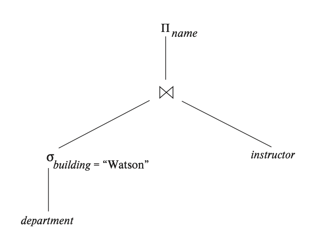
If the materialization method is to be applied, we start evaluating from the lowest-level operations of the tree, using the previously introduced algorithms to perform the operations, and then store the results in temporary relations. Next, we take this temporary relation, or (if necessary) the relation originally stored in the database, and continue executing the operations at the next level. This step is repeated until the operation at the root node is completed, at which point the final result of the entire expression is obtained. The above evaluation process is called materialized evaluation.

The cost of materialized evaluation includes not only the total cost of all operations but also the cost of writing intermediate results to disk. We assume that the records of intermediate results are stored in a buffer, and when the buffer is full, they are written to disk. The number of blocks written to disk is $b_r \approx \dfrac{n_r}{f_r}$ , where $n_r$ and $f_r$ are the number of tuples in the result relation $r$ and the blocking factor (i.e., the number of tuples that can be stored in one block), respectively. The number of disk seeks is $\lceil \dfrac{b_r}{b_b} \rceil$ , where $b_b$ is the size of the output buffer.

If double buffering is used (using two buffers, one to continue executing the algorithm while the other writes data to disk, thereby achieving parallelism between CPU activity and I/O activity), the algorithm can be executed more efficiently. The number of seeks can be reduced by allocating additional blocks to the output buffer.

Pipelining

The benefits of creating a pipeline for operations include:

Eliminating the cost of reading from and writing to temporary relations, thereby reducing the cost of query evaluation.
If the root operator in the query evaluation plan is pipelined with its inputs, query results can be generated quickly.

Implementation

The execution methods of the pipeline include:

Demand-driven pipeline (iterator model):
- The system repeatedly requests tuples from the top operation of the pipeline.
- Whenever an operation receives a tuple request, it computes the next (or next batch of) tuple(s) to be returned and returns them.
- If the operation’s input is not pipelined, it can compute the subsequent tuples to be returned based on the input relationship, while the system records the state of the data already returned.
- If there is a pipelined input, the operation also sends a tuple request to its pipeline input end.
- Using the tuple data obtained from the pipeline input end, the operation computes the output result and passes it upward to the parent operation.
Producer-driven pipeline:
- Operations do not wait for requests to generate tuples; instead, they actively and proactively generate tuples.
- Each operation is modeled as an independent process or thread within the system, which obtains a stream of tuples from its pipeline input and generates a corresponding stream of tuples for the output.

Their specific implementation methods are as follows:

Demand-driven pipeline:
- Each operation can be implemented as an iterator that provides the following functions: open(), next(), and close().
- After calling open(), each call to next() returns the next output tuple of the operation. The implementation of the operation correspondingly calls open() and next() on its inputs to obtain its input tuples when needed. The function close() is used to inform the iterator that no more tuples are needed.
- The iterator maintains its state unchanged during execution, so that consecutive next() requests receive consecutive result tuples.
Producer-driven pipeline:
- The system creates a buffer for each pair of adjacent operations to temporarily store tuples passed from one operation to the next. The processes or threads corresponding to different operations execute concurrently.
- Each operation at the bottom of the pipeline continuously generates output tuples and stores them in the output buffer until the buffer is full.
- Operations at other levels of the pipeline obtain input tuples from the lower level and generate output tuples until their output buffer is full.
- Whenever an operation consumes a tuple from the pipeline input, it removes that tuple from its input buffer.
- In either case, once the output buffer is full, the operation pauses and waits for the parent operation to extract tuples from the buffer to free up space. At this point, the operation continues generating new tuples until the buffer is full again. This process repeats until all output tuples have been generated.

Evaluation Algorithms

Query plan annotations mark edges that are pipelined, which are referred to as pipelined edges. In contrast, non-pipelined edges are called blocking edges or materialized edges.

Two operations connected by a pipelined edge must execute concurrently, with one consuming tuples while the other produces them.

A query plan can be partitioned into multiple subtrees, each containing only pipelined edges, while the edges between subtrees are non-pipelined. These subtrees are called pipeline stages. The query processor executes one pipeline stage at a time, running all operations within a single pipeline stage concurrently.

Some operations, such as sorting, are inherently blocking operations: they may not output any results until all input tuples have been examined.

However, blocking operations can consume tuples while generating them, and can output tuples to their consumers as they are produced.
Other operations, such as joins, are not inherently blocking, but their evaluation algorithms may be blocking. For example, the index nested loop join algorithm can output result tuples while fetching outer relation tuples. Thus, it is pipelined on the outer (left) relation; however, it is blocking on the index (right) input because the index must be fully built before the index nested loop join algorithm can execute.
Both inputs of the hash join algorithm are blocking operations, as it requires its inputs to be fully retrieved and partitioned before any tuples can be output. However, the hash join partitions each input and then performs multiple build-probe steps, one for each partition.

Below are two figures: the left figure shows a query that joins two relations, r and s, and then aggregates the result; the right figure shows the pipelined query plan using a hash join and in-memory hash aggregation.

Among them, pipelined edges are represented by ordinary lines, while blocking edges are represented by thick lines, and pipeline stages are enclosed within dashed boxes.
The hash join is split into three sub-operators: the sub-operators abbreviated as Part. partition r and s respectively; the operator abbreviated as HJ-BP performs the build and probe phases of the hash join.

Generally, for materialized edges, the cost of writing data to disk needs to be considered, and the cost of the consumer operator should include the cost of reading data from disk. However, when a materialized edge is between individual sub-operators, the materialization cost has already been accounted for in the operator cost, so there is no need to calculate it again.

In a more general case, the two inputs are likely not sorted. In this scenario, a technique called double-pipelined join can be used.

This algorithm assumes that the input tuples of both relations r and s are pipelined.
The tuples provided for the two relations are queued for processing; after all tuples of r and s are generated, special entries (referred to as $End_r$ and $End_s$ , respectively) are inserted into the queue as end-of-file markers.
For efficient evaluation, appropriate indexes should be built on relations r and s. When tuples are added, the indexes must be kept up to date.
The algorithm also assumes that the memory can accommodate both inputs. Even if these inputs are too large, the algorithm can still be used normally until the available memory is filled.

Chapter 12 Query Optimization

The core task of a database optimizer is to select the optimal execution plan for each given query.

In a typical relational database management system (DBMS), the complete query optimization process from SQL input to the generation of the final execution plan is as follows:

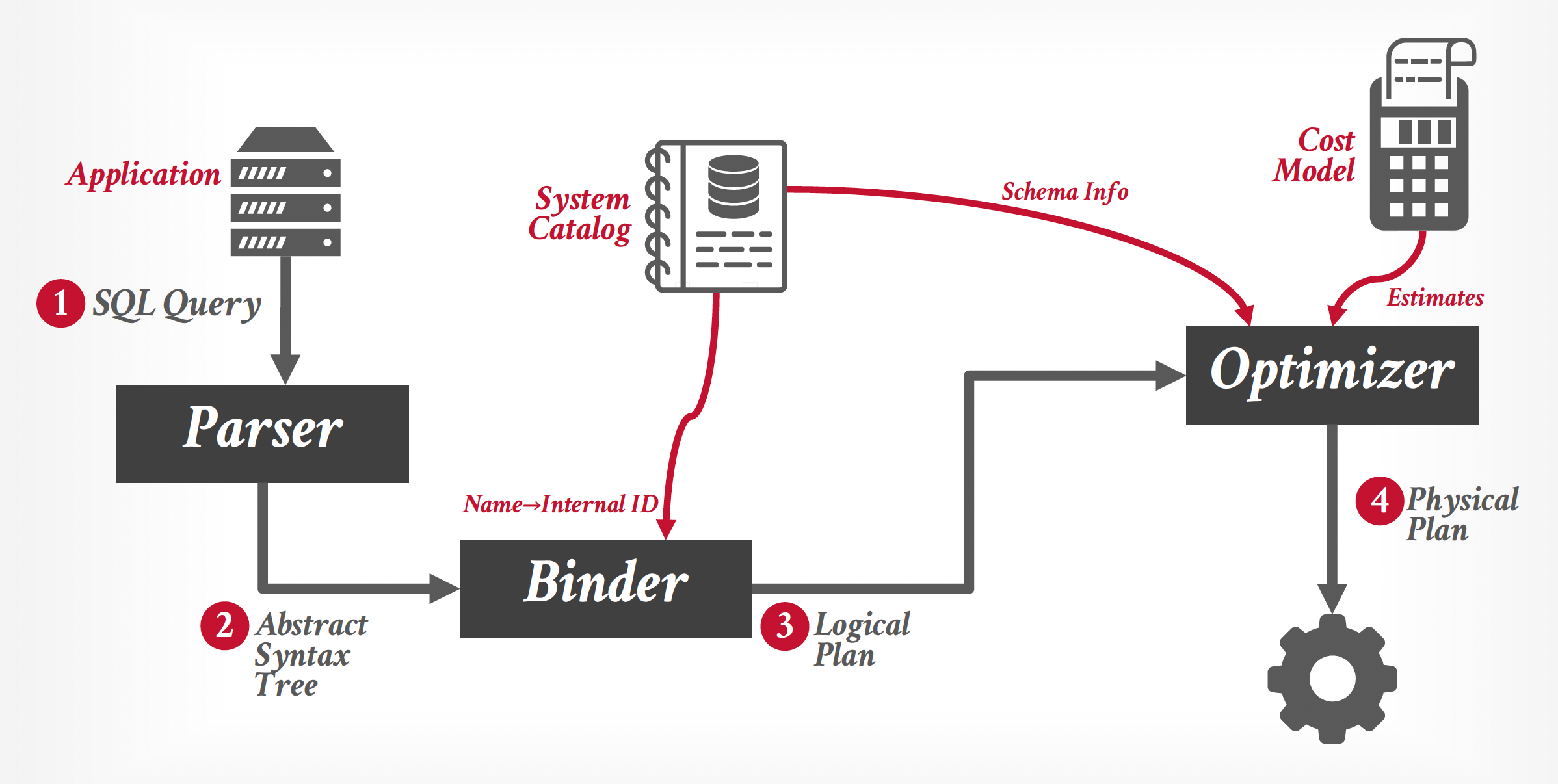
Query optimization: The process of selecting the most efficient query evaluation plan from among the many strategies that can handle a given query (especially when the query is complex). This optimization is handled by the system, which attempts to construct a query evaluation plan with the minimal cost.

Query plans can be divided into logical plans and physical plans.

The optimizer is responsible for mapping logical algebra expressions to the optimal equivalent physical algebra expressions. Logical plans roughly correspond to the relational algebra expressions in the query.
Physical operators determine the execution strategy by defining specific access paths for different operations in the query plan. The formulation of physical plans may be influenced by the physical format of the data being processed (e.g., sorting state, compression methods, etc.).

We assume that all edges in the evaluation plan graph are pipelined (unless specified as materialized), so the producer’s output is passed directly to the consumer without requiring read/write operations to disk (which materialization would require).

The steps for formulating an evaluation plan are:

Generate an expression that is logically equivalent to the given expression.
Annotate the resulting expression in alternative ways to generate other query evaluation plans.
Estimate the cost of each evaluation plan and select the one with the lowest estimated cost.

Below, we mainly introduce two major strategies for query optimization:

Static rules/heuristics: Heuristics match parts of the query with known patterns to compose a plan.
- These rules eliminate inefficiencies by transforming the query.
- Although these rules may require consulting the system catalog to understand data structures, they never need to examine the data itself.
Cost-based search: Read data and estimate the cost of executing equivalent plans; the cost model selects the plan with the lowest cost.

12.1 Transformation of Relationall Expressions

On a legal database instance, two relational algebra expressions are equivalent if they produce the same multiset of tuples.

Multiset: may contain duplicate tuples

Equivalence Rules

Symbol Conventions
Predicates: $\theta, \theta_1, \theta_2$
Attribute Lists: $L_1, L_2, L_3$
Relational Algebra Expressions: $E, E_1, E_2$

The conjunctive selection operation can be decomposed into a sequence of individual selection operations:

\sigma_{\theta_1 \wedge \theta_2}(E) \equiv \sigma_{\theta_1}(\sigma_{\theta_2}(E))

The selection operation satisfies commutativity:

\sigma_{\theta_1}(\sigma_{\theta_2}(E)) \equiv \sigma_{\theta_2}(\sigma_{\theta_1}(E))

In a sequence of projection operations, only the last (outermost) projection operation is effective; all others are ignored:

\Pi_{L_1} (\Pi_{L_2}(\dots (\Pi_{L_n}(E)) \dots)) \equiv \Pi_{L_1}(E)

where $L_1 \subseteq L_2 \subseteq \dots \subseteq L_n$

Selection operations can be expressed as Cartesian product and theta join (conditional join):

\sigma_\theta (E_1 \times E_2) \equiv E_1 \bowtie_{\theta} E_2

\sigma_{\theta_1}(E_1 \bowtie_{\theta_2} E_2) \equiv E_1 \bowtie_{\theta_1 \wedge \theta_2} E_2

Theta join satisfies the commutative law:

E_1 \bowtie_\theta E_2 \equiv E_2 \bowtie_\theta E_1

Regarding the associative law of join operations:

(E_1 \bowtie E_2) \bowtie E_3 \equiv E_1 \bowtie (E_2 \bowtie E_3)

(E_1 \bowtie_{\theta_1} E_2) \bowtie_{\theta_2 \wedge \theta_3} E_3 \equiv E_1 \bowtie_{\theta_1 \wedge \theta_3} (E_2 \bowtie_{\theta_2} E_3)

Among them, $\theta_2$ only contains attributes from $E_2, E_3$ .

When the following two conditions are met, the selection operation can be distributed into the theta join operation:

All attributes of the selection condition $\theta_1$ are contained only in one of the expressions of the join operation (for example, the attributes of $E_1$ )
$\sigma_{\theta_1} (E_1 \bowtie_{\theta} E_2) \equiv (\sigma_{\theta_1}(E_1)) \bowtie_\theta E_2$
The selection condition $\theta_1$ only includes attributes of $E_1$ , and $\theta_2$ only includes attributes of $E_2$
$\sigma_{\theta_1 \wedge \theta_2} (E_1 \bowtie_{\theta} E_2) \equiv (\sigma_{\theta_1}(E_1)) \bowtie_\theta (\sigma_{\theta_2}(E_2))$

When the following two conditions are met, the projection operation can be distributed into the theta join operation:

Let $L_1, L_2$ be attribute sets from $E_1, E_2$ respectively. Suppose the join condition $\theta$ only contains attributes from $L_1 \cup L_2$ , then:
$\Pi_{L_1 \cup L_2}(E_1 \bowtie_\theta E_2) \equiv (\Pi_{L_1}(E_1)) \bowtie_\theta (\Pi_{L_2}(E_2))$
Let $L_1, L_2$ be the attribute sets from $E_1, E_2$ respectively; $L_3$ be the attributes of $E_1$ that are included in the join condition $\theta$ but not in $L_1$ ; $L_4$ be the attributes of $E_2$ that are included in the join condition $\theta$ but not in $L_2$ . Then:
$\Pi_{L_1 \cup L_2}(E_1 \bowtie_\theta E_2) \equiv \Pi_{L_1 \cup L_2}((\Pi_{L_1 \cup L_3}(E_1)) \bowtie_\theta (\Pi_{L_2 \cup L_4}(E_2)))$
The outer join operations ⟕, ⟖, ⟗ also have similar equivalence properties.

Union and intersection in set operations satisfy the commutative law, but set difference does not.

E_1 \cup E_2 \equiv E_2 \cup E_1

E_1 \cap E_2 \equiv E_2 \cap E_1

The union and intersection operations also satisfy the associative law.

(E_1 \cup E_2) \cup E_3 \equiv E_1 \cup (E_2 \cup E_3)

(E_1 \cap E_2) \cap E_3 \equiv E_1 \cap (E_2 \cap E_3)

Selection operations can be distributed over set union, intersection, and difference operations.

\sigma_\theta(E_1 \cup E_2) \equiv \sigma_\theta(E_1) \cup \sigma_\theta(E_2)

\sigma_\theta(E_1 \cap E_2) \equiv \sigma_\theta(E_1) \cap \sigma_\theta(E_2)

\sigma_\theta(E_1 - E_2) \equiv \sigma_\theta(E_1) - \sigma_\theta(E_2)

\sigma_\theta(E_1 \cap E_2) \equiv \sigma_\theta(E_1) \cap E_2

\sigma_\theta(E_1 - E_2) \equiv \sigma_\theta(E_1) - E_2

Projection operation can be distributed over set union operations:

\Pi_L(E_1 \cup E_2) \equiv (\Pi_L(E_1) \cup (\Pi_L(E_2)))

When the following conditions are met, the selection operation can be distributed over the aggregation operation: Let $G$ be the set of grouping attributes, and $A$ be the set of aggregation expressions. When $\theta$ contains only attributes from $G$ , this equivalence holds:

\sigma_\theta(_G {\large \gamma}_A (E)) \equiv\ _G {\large \gamma}_A(\sigma_\theta(E))

About the Commutativity of Join Operations:

Full outer join satisfies commutativity: $E_1$ ⟗ $E_2 \equiv E_2$ ⟗ $E_1$
Left outer join and right outer join do not satisfy commutativity, but they can be interchanged: $E_1$ ⟕ $E_2 \equiv E_2$ ⟖ $E_1$

Under certain conditions, the selection operation can be distributed over left outer join and right outer join. Specifically, when the selection condition $\theta_1$ only involves attributes of one of the expressions in the join (assumed to be $E_1$ ), the following equivalence holds:

$\sigma_{\theta_1}(E_1$ ⟕ $_\theta E_2) \equiv (\sigma_{\theta_1} (E_1))$ ⟕ $_\theta E_2) \equiv (\sigma_{\theta_1} (E_1))$
$\sigma_{\theta_1} (E_2$ ⟖ $_\theta E_1) \equiv (E_2$ ⟖ $_\theta (\sigma_{\theta_1}(E_1))$

Under certain conditions, outer joins can be replaced by inner joins: if $\theta_1$ evaluates to false or unknown when the attributes of $E_2$ are null, then the following equivalence holds:

$\sigma_{\theta_1}(E_1$ ⟕ $_\theta E_2) \equiv \sigma_{\theta_1} (E_1 \bowtie_\theta E_2)$
$\sigma_{\theta_2}(E_1$ ⟖ $_\theta E_1) \equiv \sigma_{\theta_1} (E_2 \bowtie_\theta E_1)$

(E_1 \cup E_2) \bowtie E_3 \equiv (E_1 \bowtie E_3) \cup (E_2 \bowtie E_3)

Join Ordering

A good join order is quite important for reducing the size of intermediate results, so most query optimizers focus heavily on the order of join operations.

The order of join operations can be appropriately adjusted using the equivalence rules related to joins introduced earlier.

Enumeration of Equivalent Expressions

The process of enumerating all equivalent expressions is quite costly in terms of both space and time. Therefore, the optimizer reduces costs through the following approaches:

Space: Representation techniques that allow expressions to point to shared subexpressions can significantly reduce space requirements (by avoiding redundant representation of these identical subexpressions).
Time: If the optimizer considers evaluation cost estimates, it may be able to avoid checking certain expressions, thereby significantly reducing the time required for optimization.

12.2 Estimating Statistics of Expression Results

The cost of an operation depends on the size of the input and other statistical information.

Since it is an estimation, the result given is not precise, but generally, the estimated cost is either the actual minimum cost or close to it.

Catelog Information

The database system catalog stores the following statistical information about database relations:

$n_r$ : The number of tuples in relation $r$
$b_r$ : The number of blocks containing tuples in relation $r$
$l_r$ : The byte size of a tuple in relation $r$
$f_r$ : The blocking factor of relation $r$ , i.e., the number of tuples that can be stored in one block
$V(A, r)$ $V (A, r)$ : The number of distinct values appearing in attribute $A$ $A$ of relation $r$ $r$ , with a size equal to that of $\Pi_A(r)$ $Π_{A} (r)$
- If $A$ is a superkey of $r$ , then the value of $V(A, r)$ is $n_r$
- This statistic can also be maintained for a set of attributes $\mathcal{A}$ : the size of $V(\mathcal{A}, r)$ is $\Pi_\mathcal{A}(r)$
The catalog also records statistics related to indexes, which are not elaborated here.

Most database systems update statistics during periods of low system load, so the statistics are not entirely accurate. However, if the number of updates between two statistic updates is not too large, the statistics are sufficiently precise to provide a good cost estimate.

Most databases store the distribution of each attribute value in a histogram. In a histogram, attribute values are divided into multiple ranges, and each range is associated with the tuples corresponding to the attribute values falling within that range. The following figure is an example of a histogram:

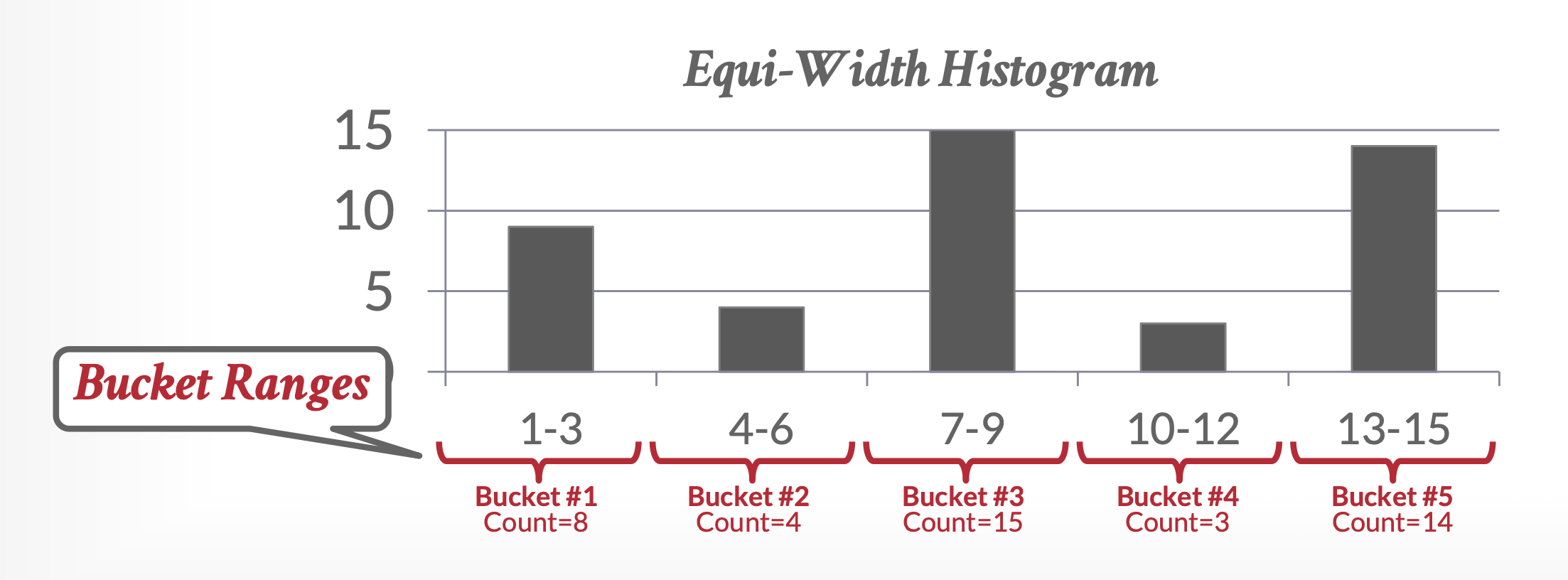
A histogram like the one shown in the figure above is an equi-width histogram, because each range has the same width. In contrast, there is also the concept of an equi-depth histogram: it adjusts the boundaries of each range so that each range contains the same number of values. Therefore, this type of histogram only stores the boundary partitions of the ranges, without needing to store the number of values in each range (whereas an equi-width histogram needs to store the total number of tuples). In summary, an equi-depth histogram provides better estimates than an equi-width histogram and uses less space (stored directly in the system catalog), making it more recommended.

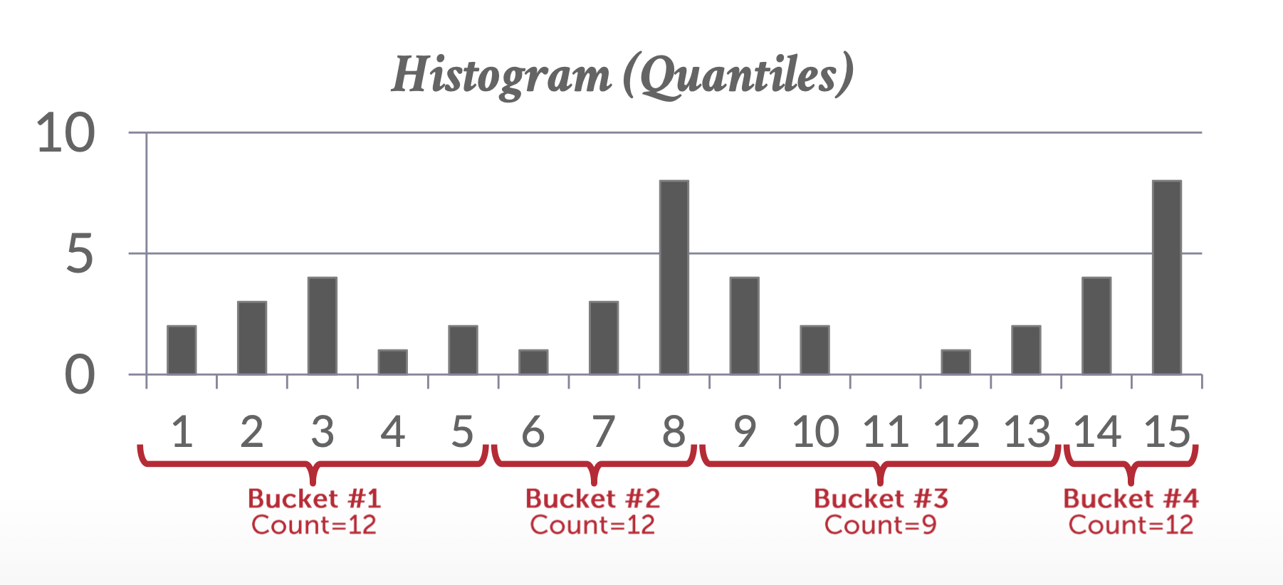
Selection Size Estimation

The evaluation of the size of the selection operation result mainly depends on the selection predicate, so the following discussion is based on different predicate scenarios:

$\sigma_{A = a}(r)$

If $a$ is a frequently occurring value, then this value can be used directly (since such a value is definitely stored).

If there is no histogram, we can only assume that the values are uniformly distributed, and the estimated size of the selection result is $\dfrac{n_r}{V(A, r)}$ tuples.

If there is a histogram for attribute $A$ , then in the formula $\dfrac{n_r}{V(A, r)}$ , $n_r$ can be replaced by the frequency count in the histogram, and $V(A, r)$ can be replaced by the number of distinct values in that range.

$\sigma_{A \le v}(r)$

Assuming the minimum values of the attributes $\min(A, r)$ and $\max(A, r)$ are both stored in the directory, and the values are uniformly distributed, the number of records can be estimated by cases:

0（ $v < \min(A, r)$ ）
$n_r$ （ $v \ge \max(A, r)$ ）
$n_r \cdot \dfrac{v - \min(A, r)}{\max(A, r) - \min(A, r)}$ ( $\min(A, r) \le v < \max(A, r)$ )

Sometimes during query optimization, the value $v$ is still unavailable. In such cases, we assume that approximately half of the records ( $\dfrac{n_r}{2}$ ) satisfy the comparison condition. Although this is quite imprecise, it serves as a temporary expedient.

Complex selection:

Conjunction ( $\sigma_{\theta_1 \wedge \theta_2 \wedge \dots \wedge \theta_n}(r)$ ): Assuming the n conditions are independent of each other, the number of tuples resulting from this selection operation is $n_r \cdot \dfrac{s_1 \cdot s_2 \cdot \dots \cdot s_n}{n_r^n}$
Disjunction ( $\sigma_{\theta_1 \vee \theta_2 \vee \dots \vee \theta_n}(r)$ ): The number of resulting tuples is:

n_r \cdot \Big[ 1 - (1 - \dfrac{s_1}{n_r}) \cdot (1 - \dfrac{s_2}{n_r}) \cdot \dots \cdot (1 - \dfrac{s_n}{n_r}) \Big]

Negation( $\sigma_{\neg \theta}(r)$ ): The number of result tuples is $n_r - \sigma_\theta(r)$ result tuples.

Join Size Estimation

The Cartesian product $r \times s$ contains $n_r \cdot n_s$ tuples, and each tuple occupies $l_r + l_s$ bytes.

Estimating the size of the result of natural join is more complicated; we will discuss it case by case:

When $R \cap S = \emptyset$ ， $r \bowtie s = r \times s$
When $R \cap S = R$ : the number of tuples in $r \bowtie s$ does not exceed the number of tuples in $s$
When $R \cap S$ $R \cap S$ does not completely include the key of either relation: we assume that each value appears with equal probability. Consider a tuple $t$ $t$ of $r$ $r$ , and let $R \cap S = \{A\}$ $R \cap S = {A}$ . We estimate that the number of tuples in $r \bowtie s$ $r ⋈ s$ related to $t$ $t$ is $\dfrac{n_s}{V(A, s)}$ $\frac{n _{s}}{V ( A , s )}$ . Then, for all tuples of $r$ $r$ , the number of tuples in $r \bowtie s$ $r ⋈ s$ is $\dfrac{n_r \cdot n_s}{V(A, s)}$ $\frac{n _{r} \cdot n _{s}}{V ( A , s )}$ .
- If there are some tuples that do not participate in the join operation, then the smaller of the estimates is more accurate.

For a theta join $r \bowtie_\theta s$ , we can first rewrite it as $\sigma_\theta(r \times s)$ , and then use the method of estimating the size of the Cartesian product and selection operation results (which has been discussed earlier) to compute it.

Size Estimation for Other Operations

Projection: The estimated value of $\Pi_A(r)$ is $V(A, r)$

Aggregation: The size of $_G {\large \gamma}_A(r)$ is $V(G, r)$

Set operations: If the two inputs of a set operation come from the same relation, we can rewrite the set operation as a disjunction, conjunction, or negation according to equivalence rules. For example, rewrite $\sigma_{\theta_1}(r) \cup \sigma_{\theta_2}(r)$ as $\sigma_{\theta_1 \vee \theta_2}(r)$ . Otherwise, the estimated size of $r \cup s$ is the sum of the sizes of $r$ and $s$ , the estimated size of $r \cap s$ is the minimum of the sizes of $r$ and $s$ , and the estimated size of $r - s$ is the size of $r$ . Obviously, these estimates are not accurate, and they are

Outer joins:

When $r$ ⟕ $s$ : size of $r \bowtie s$ + size of $r$
When $r$ ⟖ $s$ : symmetric to the previous case
When $r$ ⟗ $s$ : size of $r \bowtie s$ + size of $r$ + size of $s$

Obviously, this estimate is inaccurate, and they are all upper bounds of the accurate values.

Estimation of Number of Distinct Values

In the result of the selection operation, the number of unique values of attribute $A$ , denoted as $V(A, \sigma_\theta(r))$ , can be estimated as follows:

If the selection condition $\theta$ requires $A$ to take a specific value (e.g., $A = 3$ ), then $V(A, \sigma_\theta(r)) = 1$ .
If the selection condition $\theta$ requires $A$ to take one value from a set of specific values, then $V(A, \sigma_\theta(r))$ equals the number of specific values.
If the selection condition $\theta$ is of the form $A\ op\ v$ , where $op$ is a comparison operator, then $V(A, \sigma_\theta(r)) = V(A, r) \cdot s$ , where $s$ is the selectivity of the selection operation.
For other cases, assuming that the distribution of attribute $A$ values and the distribution of specified values in the selection condition are independent, the estimated value is $\min(V(A, r), n_{\sigma_\theta(r)})$ .

In the result of the join operation, the number of distinct values of attribute $A$ , denoted as $V(A, r \bowtie s)$ , can be estimated as follows:

If all attributes in $A$ come from $r$ , then the estimated value of $V(A, r \bowtie s)$ is $\min(V(A, r), n_{r \bowtie s})$ .

If $A$ contains attribute $A1$ from $r$ and attribute $A2$ from $s$ , then the estimated value is:

\min(V(A1, r) \cdot V(A2 - A1, s), V(A1 - A2, r) \cdot V(A2, s), n_{r \bowtie s})

12.3 Choice of Evaluation Plans

The cost-based optimizer explores the space of query evaluation plans that are equivalent to a given query and selects the one with the smallest estimated cost. If only the equivalence rules introduced earlier were used, the entire process would be quite complex. Therefore, we will consider other relatively more efficient methods below.

Cost-Based Join-Order Selection

For the join operation $r_1 \bowtie r_2 \bowtie \dots \bowtie r_n$ , there are a total of $\dfrac{(2(n-1))!}{(n-1)!}$ different join orders. It is easy to see that this number can become extremely large, making it impractical to enumerate all possible join orders.

We use a dynamic-programming algorithm to find the optimal join order, with a time complexity of $O(3^n)$ .

If a specific ordering of tuples may be useful for subsequent operations, it is called an interesting sort order. Sometimes, it is not sufficient to find the optimal join order for each subset of the given n relations. Instead, for each subset, we must find the optimal join order corresponding to the interesting sort order of the join result for that subset. For the above algorithm, the $bestplan$ array can be indexed by $[S, o]$ , where $S$ is the set of relations and $o$ is the interesting sort order. In this case, the algorithm will take the interesting sort order into account.

The above algorithm actually considers all possible ways to partition the set $S$ into two disjoint subsets twice, because each of the two subsets can play the role of $S1$ . Although considering the partition twice does not affect correctness, it wastes time. Therefore, it can be optimized as follows: find the relation $r_i$ with the smallest alphabetical order in $S1$ , and find the relation $r_j$ with the smallest alphabetical order in $S - S1$ . Execute the loop only when $r_i < r_j$ . This ensures that each partition is considered only once.

Cost-Based Optimization with Equivalence Rules

Not all queries can be optimized by obtaining the best join order, such as aggregations, outer joins, nested queries, etc. However, we can use equivalence rules to handle these operations. Since the previously introduced algorithm for enumerating equivalence rules is too costly, the following techniques will be introduced to make the algorithm more efficient:

Use a space-efficient representation of expressions to avoid generating multiple copies of subexpressions when applying equivalence rules.
Employ efficient detection techniques for repeated derivations of the same expression.
Use a dynamic programming approach based on memoization: when a subexpression is optimized for the first time, store its optimal query evaluation plan; when the same subexpression is requested for optimization later, directly return the previously saved plan.
Avoid generating all possible equivalent plans by tracking the lowest-cost plan generated for any subexpression at any given time, and prune any plan that is more expensive than the lowest-cost plan found so far.

Heuristics in Optimization

A drawback of cost-based optimization methods is the high cost of the optimization process itself. Therefore, optimizers often use heuristics to reduce optimization costs. Some heuristic rules include:

Perform selection operations as early as possible
Perform projection operations as early as possible
Optimizers that enumerate join orders typically use heuristic transformations to handle constructs other than joins, and apply cost-based join order selection algorithms only to subexpressions involving joins and selections.
Many query optimizers do not consider all possible join orders but instead restrict the search to specific join orders. For example, the System R optimizer only considers join orders where the right operand is one of the initial relations $r_1, \dots, r_n$ . This type of join order is called a left-deep join order, which is convenient for pipelined evaluation.
Oracle’s heuristic method:
- For an n-way join, it considers n evaluation plans, each using a left-deep join order starting from a different one of the n relations.
- The heuristic method builds the join order for each of the n evaluation plans by repeatedly selecting the “best” relation based on the ranking of available access paths.
- For each join, it chooses between nested-loop join or sort-merge join based on available access paths.
- Finally, the heuristic method selects one of the n evaluation plans by minimizing the number of nested-loop joins without an available index on the inner relation and the number of sort-merge joins.
A hybrid query optimization method adopted by some systems: for certain parts of a query, heuristic plan selection strategies are applied; for other parts, cost-driven selection based on generating alternative access plans is used.
For compound SQL queries (involving $\cup, \cap, -$ ), the optimizer processes each part separately and combines the evaluation plans to form a complete evaluation plan.
Most optimizers allow specifying a cost budget for query optimization. When the optimization cost budget is exceeded, the search for the optimal plan is terminated, and the best plan found so far is returned.
Plan caching: Most query optimizers optimize a query only once when it is first submitted (regardless of the constant values provided at that time) and cache the resulting execution plan as a heuristic optimization strategy. When the query is executed again later (even with new constant values), the system directly reuses the cached execution plan (only replacing the constant values). Although the optimal execution plan for the new constant values may differ from the initial plan, this heuristic method still chooses to reuse the cached plan.

Optimizing Nested Subqueries

SQL treats nested subqueries within the WHERE clause as functions that accept parameters and return a single value or a set of values. These parameters are variables from the outer query used in the nested subquery (referred to as correlation variables).

The technique of evaluating nested subqueries by treating them as function calls is known as correlated evaluation. This method is inefficient because it leads to a large number of random hard disk I/O operations. Therefore, whenever possible, the SQL optimizer attempts to convert nested subqueries into join operations; efficient join algorithms can avoid costly random I/O operations.

To correctly reflect SQL semantics, the number of duplicate tuples in the result must not be altered by rewriting—semijoin ( $r \ltimes_\theta s$ ) provides a solution for this:

Correspondingly, there is the concept of anti-semijoin (or anti-join) ( $r \overline{\ltimes}_\theta s$ ), which applies to NOT EXISTS queries.

This process of replacing nested subqueries with joins, semijoins, or anti-semijoins is called decorrelation. If aggregate operations are used in the nested subquery, this decorrelation method becomes ineffective.

It is best to avoid complex nested subqueries, as there is no guarantee that the query optimizer will successfully convert them into a form that can be evaluated efficiently.

12.4 Materialized Views

A materialized view is a view whose content is computed and stored. It constitutes redundant data because its content can be inferred from the view definition and other content in the database. In many cases, reading the content of a materialized view is much less costly than executing the query that defines the view to compute its content.

View Maintenance

One issue with materialized views is that when the data used in the view definition changes, the materialized view must be kept updated. This task is known as view maintenance. The following maintenance strategies exist:

Writing custom code → impractical
Defining triggers for insertions, deletions, and updates on the relations in the view definition; or using a simpler but more brute-force approach—fully recomputing the materialized view after each update
Modifying only the affected parts of the materialized view → incremental view maintenance
Most database systems perform immediate view maintenance: executing incremental view maintenance immediately when an update occurs, as part of the update transaction
Some database systems adopt deferred view maintenance: view maintenance is postponed, for example, collecting updates throughout the day and updating the view at night. Although this approach reduces the overhead of update transactions, it may lead to inconsistencies between the view and the underlying relations.

Incremental View Maintenance

Join Operations

Consider the materialized view $v = r \bowtie s$

If some tuples are inserted into $r$ (denoted as $i_r$ ), then $v^{new} = v^{old} \cup (i_r \bowtie s)$

If some tuples are deleted from $r$ (denoted as $d_r$ ), then $v^{new} = v^{old} - (d_r \bowtie s)$

Selection and Projection Operations

Consider the materialized view $v = \sigma_\theta (r)$

If some tuples are inserted into $r$ (denoted as $i_r$ ), then $v^{new} = v^{old} \cup \sigma_\theta (i_r)$

If some tuples are deleted from $r$ (denoted as $d_r$ ), then $v^{new} = v^{old} - \sigma_\theta (d_r)$

Handling projection operations is relatively more difficult because the result after inserting or deleting some tuples may contain duplicates. Therefore, for each tuple in the projection $\Pi_A(r)$ , we need to maintain a count for it.

If some tuples are deleted from $r$ (denoted as $d_r$ ), let $t.A$ be the projection of $t$ on attribute $A$ . We find $(t.A)$ in the materialized view, then decrement its corresponding count by 1. If the count reaches 0, we delete that tuple.

If some tuples are inserted into $r$ (denoted as $i_r$ ), and $t.A$ already exists in the materialized view, we increment its corresponding count by 1. Otherwise, we insert $(t.A)$ into the materialized view and set its corresponding count to 1.

Aggregation Operations

COUNT: Consider the materialized view $v = _G {\large \gamma}_{count(B)}(r)$

If some tuples are inserted into $r$ (denoted as $i_r$ ), first look for the group $t.G$ in the materialized view. If it does not exist, insert $(t.G, 1)$ into the materialized view; if it exists, increment the count for that group by 1.
If some tuples are deleted from $r$ (denoted as $d_r$ ), first look for the group $t.G$ in the materialized view, decrement the count for that group by 1; if the count reaches 0, delete $t.G$ from the materialized view.

SUM: Consider the materialized view $v = _G {\large \gamma}_{sum(B)}(r)$

If some tuples are inserted into $r$ (denoted as $i_r$ ), first look for the group $t.G$ in the materialized view. If it does not exist, insert $(t.G, t.B)$ into the materialized view and associate a count with it (with value 1); if it exists, add $t.B$ to the aggregate value and increment the count for that group by 1.
If some tuples are deleted from $r$ (denoted as $d_r$ ), first look for the group $t.G$ in the materialized view, subtract $t.B$ from the aggregate value, and decrement the count for that group by 1; if the count reaches 0, delete $t.G$ from the materialized view.

AVG: Consider the materialized view $v = _G {\large \gamma}_{avg(B)}(r)$

Directly updating the average after an insertion or deletion is not feasible, as it depends not only on the old average and the inserted/deleted tuples but also on the number of tuples in each group.
Therefore, maintain the aggregate values of SUM and COUNT, and compute the average by dividing the SUM value by the COUNT value.

MIN, MAX: Consider the materialized view $v = _G {\large \gamma}_{min(B)}(r)$ (the same applies to MAX, so it is not elaborated here)

Handling insertions is relatively straightforward, similar to handling SUM.
However, deletion operations can be more costly.
A good approach is to create an ordered index on $(G, B)$ , which helps efficiently find the minimum value within a group.

Other Operations

Set Intersection Operation: Consider the materialized view $v = r \cap s$

Insert a tuple into $r$ : If the tuple is also in $s$ , insert it into the view.
Delete a tuple from $r$ : If the tuple exists in the intersection, remove it from the intersection.

Outer Join: The handling method is similar to the join operation, but some additional work is required.

Delete a tuple from $r$ : Also handle those tuples in $s$ that no longer match any tuple in $r$ .
Insert a tuple into $r$ : Also handle those tuples in $s$ that previously did not match any tuple in $r$ .

Expressions

The above only considers single-step operations. To handle complete expressions, we can first calculate the incremental changes in the results for each sub-expression, and then obtain the complete incremental update.

Query Optimizations and Materialized Views

In materialized views, we can optimize queries in the following ways:

Rewrite queries using materialized views
Replace the use of materialized views with view definitions

Chapter 13 Transactions

Transaction: A single or multiple sequence of operations executed on a shared database, serving as a fundamental unit for achieving some higher-level functionality.

The four properties of a transaction—ACID—correspond to:

Atomicity: All statements in a transaction either take effect on the data entirely, or none of them do.
Consistency: If each transaction is consistent and the database is in a consistent state at the start of a transaction, it is guaranteed that the database will remain consistent upon the transaction’s completion.
- Database Consistency: The database accurately reflects the real-world entities it models and adheres to integrity constraints.
- Transaction Consistency: If the database is consistent before a transaction begins, it will also remain consistent afterward. Ensuring transaction consistency is the responsibility of the application.

Data is considered consistent if it satisfies all validation rules, such as constraints, cascades, and triggers.

Isolation: Even when multiple transactions execute concurrently, the system ensures that for every pair of transactions $T_i$ , $T_j$ , it appears as if $T_j$ completes before $T_i$ begins, or $T_j$ starts after $T_i$ finishes. Thus, a transaction neither cares about nor interferes with other transactions executing concurrently.
Durability: Once a transaction successfully ends (commits), the changes made to the database should persist, even in the event of a system failure.
- To ensure durability, both the updates implemented by the transaction and the information about the updates implemented by the transaction must be written to the hard disk before the transaction ends.

13.1 A Simple Transaction Model

This chapter mainly discusses the simplest transaction model, so we stipulate:

The only operations on data are arithmetic operations.
A data item should contain only a single data value.
Transactions access data through the following two operations: read(X) and write(X).

An inconsistent state is a system state that no longer accurately reflects the state of the database that should be captured. We must ensure that such inconsistency is invisible to the database system.

Specifically, transaction atomicity can be guaranteed through the following methods:

Logging: The DBMS records all operations so that they can be undone if a transaction is aborted. It maintains undo records both in memory and on disk. For auditing and efficiency reasons, almost all modern systems use logging mechanisms.
Shadow paging: The DBMS creates copies of the pages modified by a transaction, and the transaction makes changes to these copies. Only when the transaction commits do these page changes become visible to others. This method is generally slower at runtime than log-based DBMS. However, its advantage is that if only single-threaded operations are used, no logging is required, resulting in less data written to disk when a transaction modifies the database. This also simplifies the recovery process—simply delete all pages involved in uncommitted transactions.

The database system is responsible for maintaining atomicity, specifically handled by the database’s recovery system, the details of which will be covered in the final lecture.

13.2 Storage Sturcture

In the previous chapters, we introduced the physical storage structure of databases, one classification of which is volatile memory and non-volatile memory. Here, we introduce a third type of memory—stable storage. Information stored in this type of memory is never lost.

Although such memory cannot actually be built, we approximate it through certain techniques: replicating information across multiple non-volatile storage devices with independent failure modes. This type of storage is crucial for the durability and atomicity of transactions.

13.3 States of Transactions

For those transactions that fail to complete execution successfully, we need to abort them. To ensure atomicity, an aborted transaction must not affect the database state. Therefore, any changes made to the database by the aborted transaction must be undone. This operation is called a rollback. Rollback operations are implemented based on log information.

If a transaction completes execution successfully, it can be committed. A committed transaction transitions the database to a new consistent state, which persists even in the event of a system failure. Once a transaction is committed, its effects cannot be undone by aborting. The only way to reverse its impact is to execute a compensating transaction, but this method is not always effective.

In a simple abstract transaction model, a transaction must be in one of the following states:

Active: The initial state, maintained while the transaction is executing.
Partially committed: After the last statement has been executed.
Failed: When it is discovered that normal execution can no longer proceed.
Aborted: After the transaction has been rolled back, and the database has been restored to its state prior to the transaction’s execution.
Committed: After the transaction has successfully completed execution.

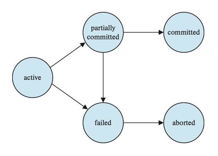
Even after all statements in a transaction have been executed, the transaction may still be aborted because the actual output is temporarily stored in main memory. Therefore, a hardware failure may prevent the successful completion of the transaction.

When a transaction enters the abort state, the system has two options:

Restart the transaction: This can be considered only if the transaction was aborted due to a hardware or software error that is not present in the internal logic of the transaction. In this case, the transaction is treated as a new transaction.
Kill the transaction: This occurs when there is an internal logic error in the transaction, requiring the application to be rewritten, or when there is bad input, or when the desired data is not found in the database.

We must carefully handle observable external writes, such as writing to the user’s screen or sending an email. Such writes cannot be undone once they occur. Most systems only allow such writes to be performed when the transaction enters the commit state. One specific implementation method is to temporarily store any values related to external writes in a special relation within the database, and only perform the actual writes when the transaction enters the commit state. If the system transaction fails after entering the commit state but before the external writes are completed, the system will continue to perform the external writes after restarting.

13.4 Serializability

Scheduling refers to the temporal order in which instructions are executed in a system. A schedule for a set of transactions must consist of all instructions from these transactions and must preserve the order in which instructions appear within each transaction.

If concurrency execution is left solely to the operating system, many possible schedules may result in inconsistent states. Therefore, a database system is needed to ensure that the executed schedule still maintains the consistent state of the database.

We can ensure consistency during concurrent execution in a database by guaranteeing that any executed schedule has the same effect as it would have without concurrency. Such a schedule is called a serializable schedule.

Suppose there is a schedule S with two consecutive instructions I and J, corresponding to transactions Ti and Tj (i != j). If I and J reference different data items, these two instructions can be swapped without affecting the schedule’s outcome. However, if I and J reference the same data item Q, their order becomes important. Consider three cases:

Both are Read: The order does not matter; it is irrelevant which one reads first.
One Read and one Write: The order must be considered.
Both are Write: Although the order of the two instructions does not affect their respective transactions, it will affect the result of the next read(Q).

In summary, for I and J, if they are operations from different transactions on the same data item and at least one of the instructions is a write operation, then we consider that a conflict occurs between I and J.

Read-Write Conflict (Unrepeatable Read): A transaction reads the same object multiple times and obtains different values.
Write-Read Conflict (Dirty Read): A transaction sees the write effects of another transaction before that transaction has committed its changes.
Write-Write Conflict (Lost Update): A transaction overwrites uncommitted data from another concurrent transaction.

If no conflicts occur, then the schedule obtained by swapping the two is equivalent to the original schedule.

If schedule S can be transformed into schedule S' by swapping a series of non-conflicting instructions—or if S and S' involve the same operations of the same transactions, and every pair of conflicting operations appears in the same order in both schedules—then S and S' are considered conflict equivalent. In particular, if schedule S is conflict equivalent to a serial schedule, then S is called conflict serializable.

It is possible for two schedules to produce the same output without being conflict equivalent.

Below is a simple and efficient method for determining the conflict serializability of a schedule: we draw a precedence graph (or dependency graph) $G = (V, E)$ for schedule S, where $V$ is the set of vertices (each vertex represents a transaction), and $E$ is the set of edges. Each edge $T_i \rightarrow T_j$ represents any of the following three conditions:

$T_i$ executes `write(Q)` before $T_j$ executes `read(Q)`
$T_i$ executes `read(Q)` before $T_j$ executes `write(Q)`
$T_i$ executes `write(Q)` before $T_j$ executes `write(Q)`

If $T_i \rightarrow T_j$ exists in the precedence graph, then in any serial schedule S' equivalent to S, $T_i$ must appear before $T_j$ .

If a cycle appears in the precedence graph, the schedule is not conflict serializable.

The serializability order of transactions is a linear order consistent with the partial order of the precedence graph. The process of finding this order is called topological sorting.

Since the definition of conflict equivalence is too strict in some cases, we may seek more relaxed forms of schedule equivalence. For example, there is a definition called view equivalence, but because it is too computationally complex, it is not actually used in practice.

13.5 Recoverability of Transactions

Now let us consider how to address the impact of transaction failures in concurrent execution. Below, we will determine which schedules are acceptable from the perspective of transaction recovery.

Recoverable Schedules

Partial schedule: does not include commit or abort operations

The definition of a recoverable schedule is: for every pair of transactions $T_i$ , $T_j$ , if $T_j$ reads data previously written by $T_i$ , then the commit of $T_i$ occurs before the commit of $T_j$ .

Cascadeless Schedules

Even if the schedule is recoverable, to correctly recover transaction $T_i$ from a failure, we may need to roll back multiple transactions. This occurs when other transactions have read data written by $T_i$ . This phenomenon, where a single transaction failure leads to a series of transaction rollbacks, is called cascading rollback.

We want to avoid cascading rollback because it incurs a significant amount of undo work. A schedule in which no cascading rollback occurs is called a cascadeless schedule. It is defined as follows: for every pair of transactions $T_i$ and $T_j$ , if $T_j$ reads a data item previously written by $T_i$ , then the commit of $T_i$ must precede the read operation of $T_j$ . Therefore, it is clear that all cascadeless schedules are recoverable.

13.6 Transcation Isolation Levels

If every transaction strictly adhered to serializability, the degree of concurrency would not be very high. In such cases, we adopt weaker consistency levels (which, of course, places an additional burden on programmers to ensure database correctness).

The SQL standard provides the following isolation levels:

Serializable: Typically ensures serializable execution, but some database systems may allow non-serializable executions when implementing this isolation level (conflict serializability falls under this category).
Repeatable Read: Only allows reading of committed data and requires that between two reads of the same data by a transaction, no other transaction is allowed to update that data.
Read Committed: Only allows reading of committed data but does not require repeatable reads.
Read Uncommitted: Allows reading of uncommitted data; it is the lowest isolation level.

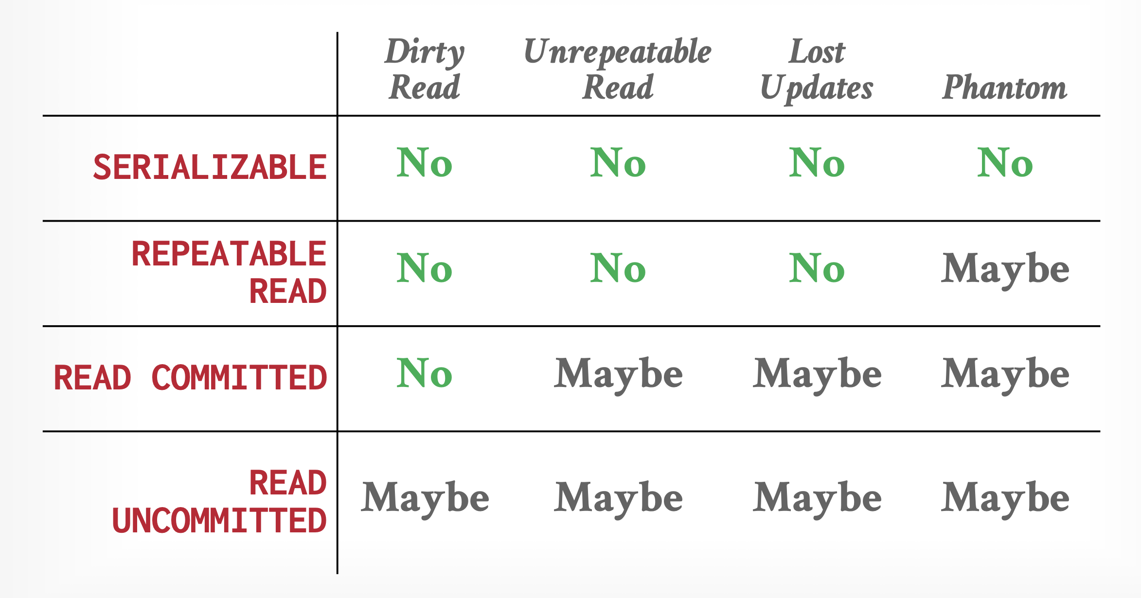
Additionally, all isolation levels prohibit dirty write operations, meaning that a transaction is not allowed to write to a data item that has already been written to by another transaction that has not yet been committed or aborted.

Many database systems operate at the read committed isolation level by default, but we can also manually set the isolation level.

13.7 Implementation of Control Concurrency

The following briefly introduces some of the most important concurrency control mechanisms, the details of which will be covered in the next lecture.

Locking

Transactions lock the data items they access, and the locking duration should be long enough to ensure serializability, but not too long, as it would otherwise excessively degrade system performance.

The next lecture mainly introduces a simple and commonly used two-phase locking protocol. As the name suggests, this mechanism requires transactions to consist of two phases: the first phase involves acquiring locks without releasing any, and the second phase involves releasing locks without acquiring any.

We can further improve this mechanism by using two types of locks:

Shared lock: Multiple transactions can simultaneously hold a shared lock on the same data item.
Exclusive lock: A transaction can hold an exclusive lock on a data item only when no other transaction holds any lock (whether shared or exclusive) on that data item.

Timestamps

At the start of each transaction, a timestamp is assigned to it. For a given data item, the system maintains two types of timestamps:

Read timestamp: retains the largest (most recent) timestamp among all transactions that have read the data item.
Write timestamp: retains the timestamp of the transaction that wrote the current value of the data item.

Timestamps are used to ensure that when transaction conflicts occur, each data item is still accessed in the order of the transaction timestamps. If a conflict cannot be avoided, the transaction causing the conflict is aborted and restarted with a new timestamp.

Multiple Versions and Snapshot Isolation

By maintaining multiple versions of data items, a transaction can read an older version of a data item instead of reading a new version written by an uncommitted transaction or a transaction that should execute later in serialization order.

Here, one widely used multi-version concurrency control technique—snapshot isolation—is introduced:

Each transaction, upon starting, has a version or snapshot of the database.
The transaction reads data from its private version, thus isolating it from updates made by other transactions.
If a transaction updates the database, the update exists only in its own version, not in the actual database. Information about the update is saved so that it can be applied to the database after the transaction commits.

Snapshot isolation ensures that reading data does not require waiting. Read-only transactions are never aborted, and only transactions that modify data have a small chance of being aborted. Since most transactions are read-only, snapshot isolation is often a major performance improvement.

However, the problem with snapshot isolation is that it provides too much isolation. In snapshot isolation, there are cases where no transaction sees the updates of another, which would not happen in serial execution and could lead to inconsistencies in the database state.

Chapter 14 Concurrency Control

The following will introduce various concurrency control schemes.

14.1 Lock-Based Protocols

Locks

One way to ensure isolation is to require that the data items being accessed follow a mutual exclusion rule: when a transaction accesses a data item, other transactions must not modify that data item. The most common method to achieve this requirement is to allow only transactions that hold a lock on the data item to access it. Various lock modes are typically provided, but we will focus on these two for now:

Shared: If transaction $T_i$ acquires a shared-mode lock (denoted as $S$ ) on data item $Q$ , then $T_i$ can read $Q$ but cannot write to $Q$ .
Exclusive: If transaction $T_i$ acquires an exclusive-mode lock (denoted as $X$ ) on data item $Q$ , then $T_i$ can both read and write $Q$ .

When a transaction accesses a data item, it makes an appropriate request to the concurrency control manager; the transaction can proceed only when the concurrency control manager grants the lock. The time between making the request and proceeding is not important, so we can assume that the transaction proceeds immediately after being granted the lock.

These two lock modes allow multiple transactions to read the same data item but restrict write access to only one transaction at a time. This characteristic can be described using a compatibility function: For any two lock modes $A$ and $B$ , if transaction $T_i$ can be immediately granted lock mode $A$ on data item $Q$ even when $Q$ already has lock mode $B$ , then modes $A$ and $B$ are said to be compatible.

Define some lock-related instructions:

lock-S(Q): Request a shared lock on data item $Q$ .
lock-X(Q): Request an exclusive lock on data item $Q$ .
unlock(Q): Unlock data item $Q$ ; this instruction does not necessarily have to be placed at the end of the transaction.

To access a data item, transaction $T_i$ must first lock it. If the data item is already locked by another transaction, the concurrency control manager will not grant the lock to $T_i$ , and $T_i$ will wait until all incompatible locks are released.

Note that a transaction must hold its lock on a data item as long as it maintains access to that data item. Moreover, even after completing the last access to the data item, the transaction cannot immediately unlock it, as this may fail to ensure serializability.

For a set of concurrently executing transactions, if no transaction can proceed further, a deadlock is said to have occurred. In such a case, one of the transactions must be rolled back to allow the others to continue. Compared to the problem of inconsistent states caused by not using locks, the consequences of deadlock may be more tolerable, as it can be resolved by rolling back a transaction, whereas inconsistent states cannot be handled by the database system.

The locking and unlocking operations of transactions must follow a set of rules called a locking protocol. Later, we will introduce some locking protocols that allow only conflict-serializable schedules. But first, we need to understand some terminology: Let $\{T_0, T_1, \dots, T_n\}$ be a set of transactions participating in schedule $S$ .

If there exists a data item $Q$ such that transaction $T_i$ holds lock mode $A$ on it, and a subsequent transaction $T_j$ holds lock mode $B$ on it, with comp(A,

Granting of Locks

Sometimes there may be a situation where there is a sequence of transactions that acquire shared locks on the same data item, and each transaction releases the lock after holding it for a while. In this case, transaction $T_i$ can never obtain an exclusive lock on that data item, so $T_i$ cannot proceed, meaning $T_i$ is in a state of starvation.

No other transaction holds a lock mode on $Q$ that conflicts with $M$
No transaction that made a request before $T_i$ is waiting to acquire a lock on $Q$

In this way, a transaction’s lock request will not be blocked by lock requests made later.

The Two-Phase Locking Protocol

A protocol that ensures (conflict) serializability is the two-phase locking protocol, which requires each transaction to issue lock and unlock requests in two phases:

Growing phase: A transaction may acquire locks (possibly after a delay), but it must not release any existing locks.
Shrinking phase: A transaction may release locks (or downgrade existing locks), but it must not acquire any new locks.

In a schedule, the point at which a transaction acquires its last lock (at the end of the growing phase) is called the lock point of that transaction. Transactions in a schedule can be ordered by their lock points, and this order corresponds to the serializable order.

This protocol does not guarantee freedom from deadlocks, and it may also lead to cascading rollbacks.

To avoid this problem, we make a slight modification to the original protocol, resulting in the strict two-phase locking protocol. This protocol, based on the original, requires that all exclusive locks held by a transaction be retained until the transaction is committed. Compared to the original protocol, it prevents cascading rollbacks and is therefore widely used in database systems.

Another variant is the rigorous two-phase locking protocol, which requires that all locks be retained until the transaction is committed. Thus, under this protocol, transactions can be serialized in commit order. This implementation is simpler and more straightforward, and it also avoids cascading rollbacks, but it reduces the degree of concurrency.

So far, the various schedules we have recognized are as follows:

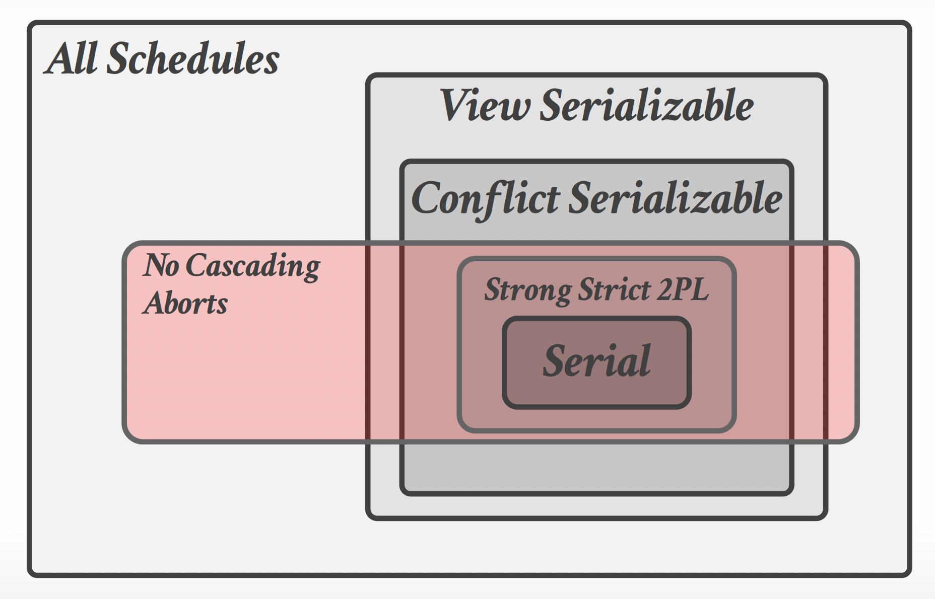
To improve concurrency, we add a lock conversion mechanism to the basic two-phase locking protocol, which supports:

Upgrade: shared lock → exclusive lock, occurring only in the growing phase
Downgrade: exclusive lock → shared lock, occurring only in the shrinking phase

It is important to note that when a data item $Q$ is locked by other transactions in shared mode, a transaction attempting to upgrade its lock on $Q$ will be forced to wait.

Similar to the basic two-phase locking protocol, two-phase locking with lock conversion only generates conflict-serializable schedules, and transactions can be serialized at their lock points.

Below is a simple and commonly used locking/unlocking scheme:

When transaction $T_i$ initiates a read(Q) operation, the system issues a lock-S(Q) instruction after that operation.
When transaction $T_i$ $T_{i}$ initiates a write(Q) operation, the system checks whether $T_i$ $T_{i}$ already holds a shared lock on $Q$ $Q$ :
- If so, the system issues an upgrade(Q) instruction after write(Q).
- Otherwise, the system issues a lock-X(Q) instruction after write(Q).
After the transaction commits or aborts, all locks acquired by that transaction are released.

Implementation of Locking

The lock manager can be implemented as a process that receives information from transactions and responds by sending messages. Specifically:

Grant lock information or send information requesting a transaction rollback (when a deadlock occurs) as a response to lock request information.
For unlock information, only an acknowledgment is required, but lock grant information may need to be sent to other waiting transactions.

The lock manager uses the following data structures:

For each currently locked data item, maintain a linked list of records, each representing a request, following the order in which the requests arrive.
Use a hash table (referred to here as the lock table, which uses overflow chains) indexed by the data item name to locate the corresponding linked list for the data item. A schematic diagram of the lock table is shown below.

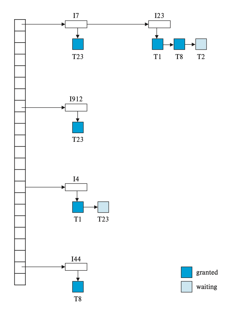
The lock manager process initiates requests in the following manner:

When a lock request message arrives, if the linked list corresponding to the data item exists, the record is added to the end of the list; otherwise, a new linked list containing the request record is created.
- When a data item is not locked, the lock manager grants the lock request; however, if it is locked, the lock manager grants the request only if the requested lock is compatible with the current lock; otherwise, the request must wait.
When an unlock message is received, the lock manager deletes the data item record from the linked list corresponding to the transaction. It then tests the subsequent record (if any) to see if the request can now be granted; if so, the lock manager grants the request. It then continues processing subsequent records in the same manner, and so on.
If a transaction is aborted, the lock manager deletes any pending requests initiated by that transaction. Once the database system takes appropriate actions to undo the transaction, the lock manager releases all locks held by the aborted transaction.

This approach prevents the problem of transaction starvation.

Graph-Based Protocols

In addition to the two-phase locking protocol, there are other types of protocols, but they require some additional information, which can be described using various models. The simplest model requires us to know in advance the order in which data items are accessed. To obtain such information in advance, a partial order $\rightarrow$ over all data items $D = \{d_1, d_2, \dots, d_n\}$ is needed. If $d_i \rightarrow d_j$ , then any transaction that accesses $d_i$ and $d_j$ must first access $d_i$ and then access $d_j$ . This partial order can be realized through the logical or physical organization of the data, or solely for concurrency control purposes.

The partial order indicates that we can view $D$ as a directed acyclic graph, which we call the database graph. For simplicity, we restrict this graph to the form of a rooted tree; the corresponding protocol is called the tree protocol. The only locking instruction used in this protocol is lock-X. Each transaction $T_i$ locks a data item at most once and must follow these rules:

Let the first lock of $T_i$ be on any data item.
Subsequently, a data item $Q$ can be locked by $T_i$ only if the parent of $Q$ is already locked by $T_i$ .
Data items can be unlocked at any time.
A data item that has been locked or unlocked by $T_i$ cannot be locked again by $T_i$ .

All schedules that are legal under the tree protocol are conflict serializable.

To make the tree protocol recoverable and cascadeless, a slight modification can be made: do not allow the release of exclusive locks until the transaction ends. However, this approach reduces the degree of concurrency. Another method to increase concurrency, but only ensures recoverability, is:

For each data item with an uncommitted write operation, we record which transaction last performed a write operation on that data item.
Whenever a transaction $T_i$ reads an uncommitted data item, we record a commit dependency of $T_i$ on the transaction that last wrote that data item.
Thereafter, $T_i$ is not allowed to commit until all transactions on which it depends have completed their commits.
If any of these dependent transactions aborts, then $T_i$ must also be aborted.

The advantage of the tree protocol is that it ensures no deadlocks occur, thus eliminating the need for rollback. Another advantage is that unlock operations can be performed earlier, thereby reducing waiting time and improving concurrency. However, its disadvantages include increased locking overhead, potential additional waiting time, and a possible decrease in concurrency.

In fact, there exist schedules that follow the two-phase locking protocol but do not follow the tree protocol, and vice versa.

14.2 Deadlock Handling

If there exists a set of waiting transactions $\{T_0, T_1, \dots, T_n\}$ such that $T_0$ is waiting for data locked by $T_1$ , $T_1$ is waiting for data locked by $T_2$ , …, $T_{n-1}$ is waiting for data locked by $T_n$ , and $T_n$ is waiting for data locked by $T_0$ , then we consider these transactions to be in a deadlock state.

The following are two main approaches to handling deadlock problems:

Deadlock prevention: ensuring that the system never enters a deadlock state
Deadlock detection and recovery: allowing the system to enter a deadlock state, but then attempting to recover from it

If deadlocks are likely to cause relatively high losses, deadlock prevention can be adopted; otherwise, the more efficient deadlock detection and recovery can be used.

Deadlock Prevention

By ordering lock requests or requiring all locks to be acquired at once, ensure that no circular wait occurs.

The simplest approach is to require each transaction to lock all data items it will use before execution begins. However, this method has the drawbacks of difficulty in predicting which data items need to be locked and low utilization of data items.
Enforce an ordering of data items and require transactions to lock data items only in a sequence consistent with that order.
A variant of the above method uses a total order of data items and two-phase locking. Once a transaction locks a specific data item, it cannot request locks on data items that precede it in the order. The main advantage of this method is its ease of implementation.

Similar to deadlock recovery, when a transaction’s waiting could lead to a deadlock, roll back the transaction instead of continuing to wait.

This is specifically achieved through preemption: when transaction $T_j$ requests a lock on a data item already locked by $T_i$ , the lock is taken from $T_i$ by rolling back $T_i$ , and then the lock is granted to $T_j$ .
To control preemption operations, we assign a timestamp (based on a counter or system clock) to each newly started transaction. The system uses timestamps solely to decide whether a transaction should wait or be rolled back. If a transaction is rolled back, its old timestamp is retained when it is restarted. Two different schemes using timestamps are given below:
- Wait-die (non-preemptive technique): When transaction $T_i$ requests a lock on a data item already locked by $T_j$ , $T_i$ can wait only if its timestamp is smaller than that of $T_j$ ( $T_i$ is older than $T_j$ ); otherwise, $T_i$ must be rolled back.
- Wound-wait (preemptive technique): When transaction $T_i$ requests a lock on a data item already locked by $T_j$ , $T_i$ can wait only if its timestamp is greater than that of $T_j$ ( $T_i$ is newer than $T_j$ ); otherwise, $T_j$ must be rolled back ( $T_j$ is “wounded” by $T_i$ ).

A common problem with both methods is that they can cause unnecessary rollbacks.

Method based on lock timeout: A transaction requesting a lock waits for at most a certain amount of time. If the lock is not granted to the transaction within this period, the transaction is considered to have timed out and must be rolled back and restarted.

This method is easy to implement and is effective when transactions are not too complex and long waits may lead to deadlocks.
However, it is difficult to determine an appropriate timeout duration: waiting too long introduces unnecessary delays, while waiting too little leads to unnecessary rollbacks, resulting in resource waste. Additionally, this method may cause transactions to starve. Therefore, its application is limited.

Deadlock Detection and Recovery

Maintain information about the data items currently assigned to transactions, as well as any outstanding requests for data items.

Provide a detection algorithm that uses the above information to determine whether the system has entered a deadlock state. We also need to consider when to invoke the algorithm—this depends on two factors: the frequency of deadlock occurrences and the number of transactions affected by deadlocks.

When the detection algorithm determines that a deadlock exists, recovery from the deadlock involves the following three steps:

Victim Selection: For a given set of transactions, we must decide which transaction to roll back (referred to as the victim) to break the deadlock. Generally, we choose the transaction with the smallest rollback cost, but this minimum cost is difficult to define precisely. The cost of rollback needs to consider the following factors: the time the transaction has already spent computing, the number of data items used by the transaction, how many more data items are needed to complete the transaction, and the number of transactions involved in the rollback.
Rollback: The simplest approach is total rollback: abort the transaction and restart it. However, partial rollback is more efficient, rolling back only the part of the transaction necessary to break the deadlock. But this method requires the system to maintain additional information about the state of all running transactions—specifically, the sequence of lock requests and grants, as well as updates performed by the transaction, must be recorded.
Starvation: It is possible that the same transaction is always chosen as the victim, in which case it can never complete its task, leading to a starvation problem. Therefore, we must ensure that a transaction is not selected as a victim more than a specified number of times. The most common solution is to include the number of rollbacks in the cost factor.

A deadlock situation can be represented using a directed graph called a wait-for graph, denoted as $G = (V, E)$ , where:

Vertices represent transactions in the system, and edges represent ordered pairs $T_i \rightarrow T_j$ , indicating that transaction $T_i$ is waiting for transaction $T_j$ to release the lock on a data item it needs.
When transaction $T_i$ requests a lock on a data item that is currently locked by $T_j$ , the edge $T_i \rightarrow T_j$ is inserted into the graph; when $T_j$ no longer holds the lock on that data item, the edge is removed.
A deadlock exists in the system if and only if there is a cycle in the wait-for graph. To detect deadlocks, the system needs to maintain the wait-for graph and periodically invoke an algorithm that searches for cycles in the graph.

14.3 Multiple Granulartiy

In the concurrency control schemes introduced earlier, we have always treated individual data items as synchronization units. However, sometimes grouping multiple data items together and treating them as a single synchronization unit can yield better results. For example:

Suppose a transaction $T_i$ needs to access an entire relation table, and the locking protocol used is to lock individual tuples. Then $T_i$ must lock every tuple in that relation table. Clearly, acquiring a large number of such locks is time-consuming; worse still, the lock table may become extremely large and unable to fit in memory.
It would be more efficient if $T_i$ could directly lock the entire relation table with a single lock request. Conversely, if a transaction $T_j$ only needs to access a small number of tuples, it should not be forced to lock the entire relation table, as this would lose the benefits of concurrency.

Therefore, we need a mechanism that allows the system to define multiple levels of granularity: that is, to allow data items to have variable sizes; and to define a hierarchy of data granularity, where smaller granularities are contained within larger ones. Such a hierarchy can be represented by a tree, as shown below:

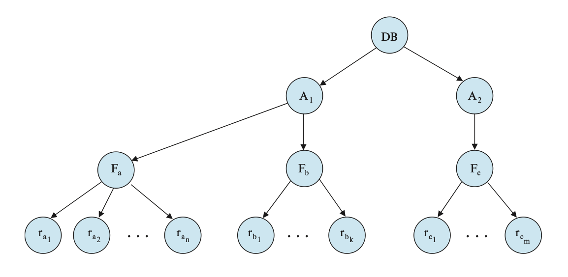
Unlike independent nodes in a tree protocol, the non-leaf nodes of a multi-granularity tree represent data associated with their descendants.
The topmost node in the tree represents the entire database.
The second-level nodes represent areas, and it can be seen that the database consists of multiple areas.
Each area contains multiple files, reflected in the tree as file nodes being descendants of area nodes; note that files must not span multiple areas.
Each file contains multiple records, as descendants of file nodes; similarly, records must not exist in multiple files.
Each node can be locked individually. When a transaction locks a node (whether with a shared lock or an exclusive lock), it implicitly locks all its descendants.
If transaction $T_j$ wants to lock record $r_b$ , it must traverse from the root of the tree. If it finds a node on the path with a lock incompatible with $T_j$ ‘s lock, then $T_j$ ‘s locking operation must be delayed.

If transaction $T_k$ wants to lock the entire database, but another transaction $T_i$ has already locked a subtree, it must determine whether locking is possible before proceeding. Traversing the entire tree could solve this problem, but this brute-force method is too inefficient to be acceptable. Therefore, we adopt a more efficient approach called intention lock modes: if a node is locked with an intention lock, its descendants are explicitly locked. Thus, a transaction does not need to traverse the entire tree—if it wants to lock node $Q$ , it only needs to traverse the path from the root to $Q$ .

Intention locks can be associated with shared locks or exclusive locks, leading to additional lock modes:

Intention-shared (IS) mode: explicitly locks descendants of a node with shared locks.
Intention-exclusive (IX) mode: explicitly locks descendants of a node with shared or exclusive locks.
Shared and intention-exclusive (SIX) mode: the root of the subtree under this node is explicitly locked with a shared lock, while lower-level nodes are explicitly locked with exclusive locks.

Including the general shared and exclusive locks, we obtain the following compatibility function:

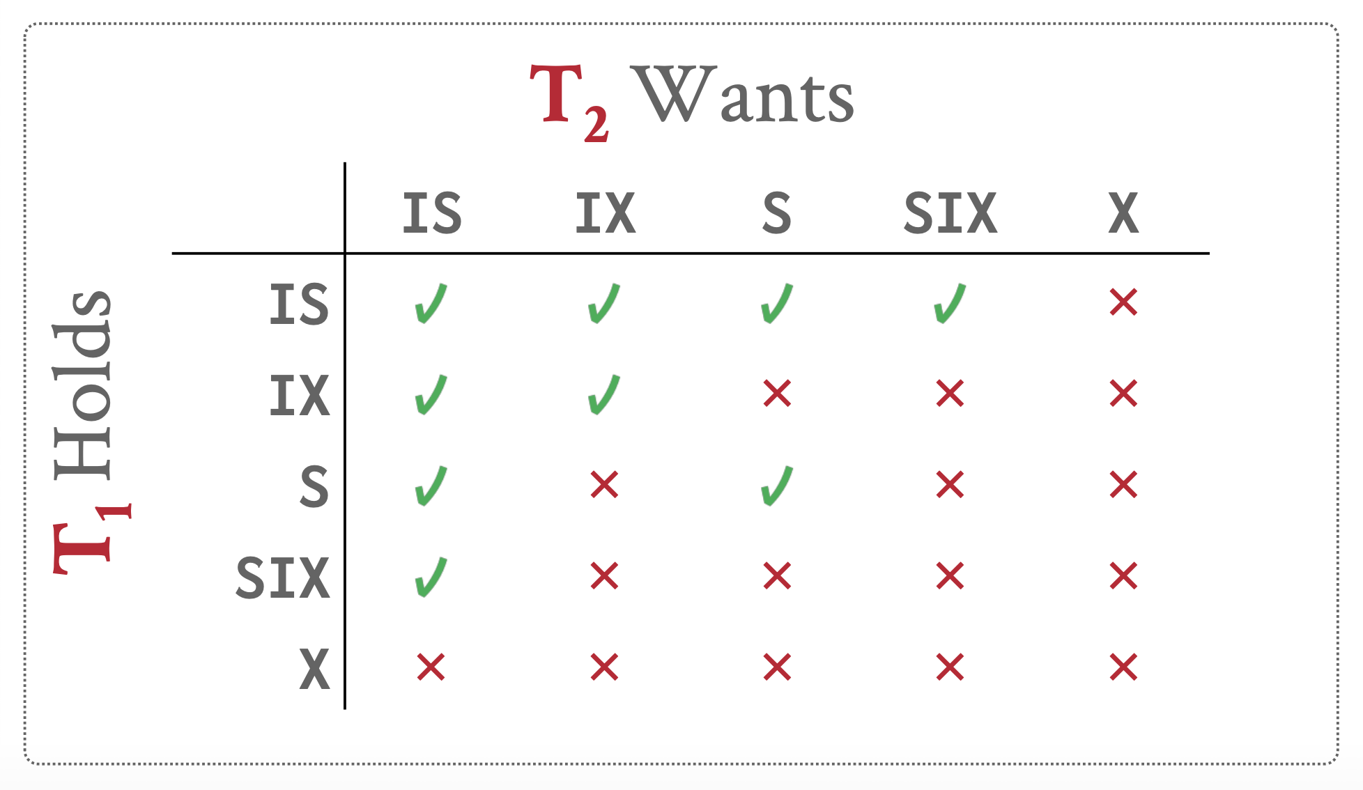
Based on the concept of multi-granularity, we can derive the multiple-granularity locking protocol. This protocol uses the five types of locks mentioned above to ensure serializability. It requires that transaction $T_i$ must follow the rules below before locking a node $Q$ :

Ensure that $T_i$ must adhere to the compatibility function given above.
Ensure that $T_i$ must first lock the root node of the tree (using any lock mode).
$T_i$ can lock $Q$ with an S or IS lock only if $T_i$ already holds an IX or IS lock on the parent node of $Q$ .
$T_i$ can lock $Q$ with an X, SIX, or IX lock only if $T_i$ already holds an IX or SIX lock on the parent node of $Q$ .
$T_i$ can lock a node only if it has not previously unlocked any node.
$T_i$ can unlock $Q$ only if it does not hold any locks on the children of $Q$ .

It can be seen that the multiple-granularity locking protocol requires locks to be acquired in a top-down (root-to-leaf) order, while locks are released in a bottom-up (leaf-to-root) order.

The multiple-granularity locking protocol does not guarantee freedom from deadlocks.

The advantage of this protocol is that it enhances concurrency and reduces lock overhead. It is particularly suitable for scenarios such as short transactions that access only a few data items, and long transactions that generate reports from single or multiple files.

The number of locks required by an SQL query can typically be estimated based on the results of relational scan operations. For example, a relation scan acquires a single lock at the relation level, while an index scan may acquire an intention lock at the relation level and impose regular locks at the tuple level. If a transaction acquires a large number of tuple locks, it may cause the lock table to become overly full. In such cases, the lock manager can implement a lock escalation mechanism—replacing multiple low-level locks with a single higher-level lock; in the example above, a single relation-level lock can replace a large number of tuple-level locks.

14.4 Operations

Now we consider more operations:

delete(Q): Delete data item $Q$ from the database

insert(Q): Insert a new data item $Q$ into the database and assign an initial value to $Q$

Deletion

To understand how the delete instruction affects concurrency control, we must determine when delete conflicts with other instructions. Let $I_i, I_j$ be instructions of transactions $T_i, T_j$ respectively, which appear in consecutive order in schedule $S$ ; and let $I_i$ = delete(Q). Next, we discuss based on $I_j$ :

If $I_j$ = read(Q): $I_i, I_j$ conflict. If $I_i$ appears before $I_j$ , $T_j$ will have a logical error; if $I_j$ appears before $I_i$ , $T_j$ can successfully execute the read operation.
If $I_j$ = write(Q): $I_i, I_j$ conflict. If $I_i$ appears before $I_j$ , $T_j$ will have a logical error; if $I_j$ appears before $I_i$ , $T_j$ can successfully execute the write operation.
If $I_j$ = delete(Q): $I_i, I_j$ conflict. If $I_i$ appears before $I_j$ , $T_j$ will have a logical error; if $I_j$ appears before $I_i$ , $T_i$ will have a logical error.
If $I_j$ = insert(Q): $I_i, I_j$ conflict. Assume data item $Q$ does not exist before the execution of $I_i, I_j$ . Then if $I_i$ appears before $I_j$ , $T_j$ will have a logical error; if $I_j$ appears before $I_i$ , there is no logical error. Similarly, if data item $Q$ exists before the execution of $I_i, I_j$ , a logical error occurs when $I_j$ appears before $I_i$ , and not otherwise.

Thus:

In the two-phase locking protocol, an exclusive lock must be acquired for a data item before it is deleted.
In the timestamp ordering protocol, a test similar to the write check must be performed. Suppose $T_i$ issues a delete(Q) instruction:
- If TS( $T_i$ ) < R-timestamp( $Q$ ), then the value of $Q$ has already been read by another transaction $T_j$ with TS( $T_j$ ) > TS( $T_i$ ). Therefore, the delete operation is rejected, and $T_i$ is rolled back.
- If TS( $T_i$ ) < W-timestamp( $Q$ ), then another transaction $T_j$ with TS( $T_j$ ) > TS( $T_i$ ) has already written to $Q$ . Therefore, the delete operation is rejected, and $T_i$ is rolled back.
- Otherwise, the delete operation is executed.

Insertion

As mentioned earlier, the insert(Q) operation and the delete(Q) operation conflict; in addition, insert(Q) also conflicts with read(Q) and write(Q), because read and write cannot be performed on a non-existent data item.

In the two-phase locking protocol, if $T_i$ performs the insert(Q) operation, then $T_i$ must acquire an exclusive lock on the newly created data item $Q$ .
In the timestamp ordering protocol, if $T_i$ performs the insert(Q) operation, then R-timestamp(Q) and W-timestamp(Q) are set to TS( $T_i$ ).

Predicate Reads and the Phantom Phenomenon

Phantom phenomenon (also known as phantom read): When a transaction executes the same query multiple times (predicate read) during its execution, but due to other concurrent transactions inserting or deleting new records that meet the query conditions, the result set of the later query differs from that of the previous query, as if “phantoms” have appeared. These newly appearing or disappearing records are the “phantoms.”

There are several solutions:

Re-execute scan: The DBMS records the WHERE clauses of all queries executed by the transaction. When the transaction commits, it may re-execute the queries to check whether the results differ. This can detect changes caused by newly added or deleted records, ensuring consistency of the results.
Predicate locking: Locks are acquired based on the query predicate to ensure that no data satisfying the predicate is modified by other transactions. However, this method is rarely used.

Index Locking

Avoid locking the entire index: any transaction that inserts a tuple into a relation must insert corresponding information into the index; phantom phenomena are eliminated by applying a locking protocol on the index.

The specific operations of the index-locking protocol are as follows:

Each relation must have at least one index.
A transaction $T_i$ can access a tuple only if it is found through one or more indexes on the relation. In the index-locking protocol, a relation scan is treated as scanning all leaf nodes in the index.
A transaction $T_i$ performing a search must acquire shared locks on all nodes in the index it accesses.
When a transaction $T_i$ performs an insert, delete, or update operation on a tuple $t_i$ in relation $r$ , it must simultaneously update all indexes on $r$ . The transaction needs to acquire exclusive locks on all index leaf nodes affected by the insert, delete, or update operation. Specifically:
- Insert/Delete: The affected leaf nodes are those that (after insertion) will contain the search key value of the tuple or (before deletion) contained the search key value of the tuple.
- Update: The affected leaf nodes include two types—nodes that contained the old search key value before modification and nodes that will contain the new search key value after modification.
Lock acquisition for tuples follows the usual rules.
The rules of the two-phase locking protocol must be followed.

Specific schemes for index locking include:

Key-value locks: Locking a single key-value pair in the index, including virtual keys for non-existent values.
Gap locks: Locks on the gaps between key-value pairs, preventing insertions into these gaps.
Key-range locks: Locking a range of keys, from an existing key to the next key.
Hierarchical locks: Allowing transactions to hold broader key-range locks in different modes, reducing the overhead of the lock manager.

It should be noted that the index-locking protocol does not address concurrency control for internal nodes in the index.

Locking index leaf nodes can prevent any update operations on the nodes, even if the update operation does not actually conflict with the predicate.

Chapter 15 Recovery System

Recovery algorithms refer to techniques that ensure database consistency, transaction atomicity, and durability, safeguarding data even in the event of a failure. When a system crashes, all committed data in memory that has not yet been written to disk faces the risk of loss, which clearly contradicts user expectations—they assume that successfully committed data changes should be permanently preserved. The core function of recovery algorithms is precisely to prevent information loss after a crash. Each recovery algorithm consists of the following two parts:

Actions taken during normal transaction processing to ensure sufficient information is available for recovery
Actions taken after a failure to restore the database content, ensuring database consistency, atomicity, and durability

15.1 Failure Classification

Transaction failure: divided into the following two categories:

Logical error: The transaction cannot continue normal execution due to internal conditions (such as bad input, data not found, overflow, resource limits exceeded, etc.).
System error: The system enters an unexpected state (such as a deadlock), causing the transaction to be unable to continue normal execution; however, the transaction can be re-executed later.

System crash: Problems with hardware, database software, or the operating system cause the loss of volatile memory contents and stop transaction processes, while the contents of non-volatile memory remain unaffected (this assumption is called the fail-stop assumption).

Disk failure: Due to a disk head crash or a failure during data transfer, the contents of a disk block are lost. In this case, the contents must be restored using other disks or archival backups from third-party media.

15.2 Storage

Stable-Storage Implementation

To achieve stable storage, we need to replicate the required information multiple times and store it in different non-volatile storage media with independent failure modes. Additionally, we must update the information in a controlled manner to ensure that failures occurring during data transmission do not corrupt the required information.

The RAID system mentioned earlier seems well-suited for this task, but it is not a perfect solution—it cannot withstand external disasters such as fires, floods, etc. Therefore, many systems adopt archival backup measures (e.g., storing data on media like tape). However, this method cannot continuously back up data, so the most recent data may still be lost in the event of a disaster. This leads to another approach—remote backup, which involves copying the data from stable storage to a remote location via a computer network.

When transferring data between memory and disk, one of the following outcomes occurs:

Successful completion: The transmitted information successfully reaches its destination.
Partial failure: A failure occurs during transmission, resulting in incorrect information in the target block.
Total failure: A failure occurs early enough during transmission that the content of the target block remains intact.

When a data-transfer failure occurs, the system should be able to detect the failure and invoke a recovery process to restore the data block to a consistent state. To achieve this, the system must maintain two physical blocks for each logical database block.

In a mirrored disk scheme, the two blocks are located at the same site.
In a remote backup scheme, one block is local, and the other is at a remote site.

The steps for executing an output operation are as follows:

Write the information to the first physical block.
When the first write operation completes successfully, write the same information to the second physical block.
The output is considered complete only when the second write operation completes successfully.

If a failure occurs while writing a data block, the two copies may become inconsistent. During recovery, the system must check each pair of copies for every data block:

If the contents of both copies are consistent and no errors are detected, no further action is needed.
If an error is detected in one copy, the system replaces the corrupted block with the content of the other copy.
If no errors are detected in either copy but their contents differ, the system can arbitrarily choose one copy to replace the content of the other.

Regardless of the method used, the recovery process ensures that a stable storage write operation either fully succeeds (i.e., updates all copies) or leaves the original state unchanged.

The requirement to compare each pair of corresponding blocks during recovery incurs significant overhead. However, this cost can be substantially reduced by using a small amount of non-volatile RAM to track ongoing block write operations—during recovery, only those blocks with incomplete writes need to be compared.

Data Access

Data block movement between disk and main memory can be initiated through the following two operations:

input(A): Transfer physical block A to main memory
output(B): Transfer buffer block B to disk and replace the appropriate disk block

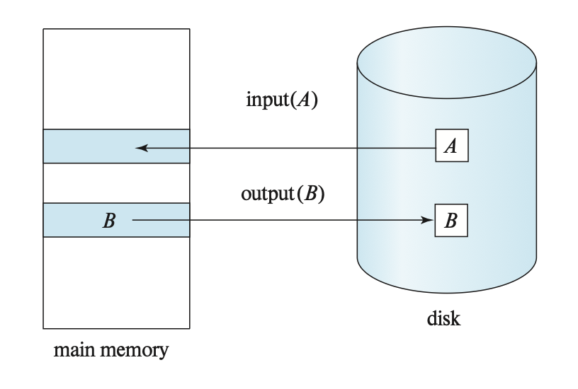
In the previous lecture, it was mentioned that each transaction $T_i$ has a private workspace used to store copies of data items that $T_i$ accesses and updates.

The system creates a workspace when a transaction starts.
When a transaction commits or aborts, the system removes it.

Each data item $X$ stored in the workspace of transaction $T_i$ is denoted as $x_i$ . Transaction $T_i$ interacts with the database system by transferring data between its workspace and the system buffer. We implement data transfer through the following two operations:

read(X): Assigns the value of data item X to the local variable $x_i$ . This process can be broken down into the following steps:
- If the data block $B_X$ containing X is not in main memory, initiate input(B_X).
- Assign the value of X in the buffer block to $x_i$ .
write(X): Assigns the value of the local variable $x_i$ to the data item X in the buffer block. This process can be broken down into the following steps:
- If the data block $B_X$ containing X is not in main memory, initiate input(B_X).
- Assign the value of $x_i$ to X in the buffer block $B_X$ .

The buffer block will eventually be written to disk, either because the buffer manager needs to free up memory space for other purposes, or because the database system wants to synchronize changes in the buffer block to the disk. When the database system issues an output(B) instruction, we say it performs a force-output operation on buffer B.

When a transaction first needs to access data item X, it must execute the read(X) operation. Subsequently, all updates to X by the transaction are performed on $x_i$ . At any point during execution, the transaction can execute write(X) to reflect the changes to X in the database; and after the final write to $x_i$ is completed, write(X) must be executed.

For the buffer block $B_X$ storing X, the output operation output(B_X) does not need to take effect immediately after write(X) is executed, because the block may also contain other data items that are being accessed. Therefore, the actual output can be delayed. It is important to note: if the system crashes after write(X) is executed but before output(B_X) is executed, the new value of X will never be written to disk and will be lost. However, in practice, database systems take additional measures to ensure that updates performed by committed transactions are not lost even in the event of a system crash.

15.3 Log-Based Recovery

To ensure the atomicity of transaction $T_i$ , we want either all modifications made by $T_i$ to the database to take effect, or none at all. To achieve this goal,

first, the information describing the modifications must be output to stable storage, rather than directly modifying the database itself. This information helps us ensure that all modifications made by committed transactions are reflected in the database.

Additionally, we need to preserve information related to the old values of the modified data items, because when the transaction that made the modification fails (aborts), this information can help us undo the changes caused by the failed transaction.

The most common method is to use a log to record such information, and the recovery scheme using this approach is called log-based recovery.

Log Records

Logs are composed of a series of log records, which document all database update activities. There are various types of log records, among which the update log record describes a single database write operation and contains the following fields:

Transaction identifier: The unique identifier of the transaction performing the write operation.
Data-item identifier: The unique identifier of the data item being written, typically the location of the data item on disk, including the identifier of the block containing the data item and the offset within the block.
Old value: The value of the data item before the write operation.
New value: The value of the data item after the write operation.

We use $<T_i, X_j, V_1, V_2>$ to represent an update log record, where these four letters correspond to the four fields mentioned above. There are also special log records that document “significant” events in transaction processing:

$<T_i \text{ start}>$ : Transaction $T_i$ starts.
$<T_i \text{ commit}>$ : Transaction $T_i$ commits.
$<T_i \text{ abort}>$ : Transaction $T_i$ aborts.

Whenever a transaction performs a write operation, a log record must be created for that write operation and added to the log before modifying the database. Once the log record exists, the modification can be output to the database if conditions permit. Additionally, the system must have the ability to undo modifications that have been output to the database, which can be achieved through rollback operations using the old value field in the log record.

Since logs are crucial for system and disk failure recovery, they must be stored in stable storage. For now, we assume that each log record is immediately appended to the end of the log in stable storage upon creation. Later, we will discuss when this requirement can be safely relaxed to reduce the overhead caused by log records.

Because logs contain a complete record of all database activities, the amount of data stored in the logs can become very large. Later, we will also explain when log information (that is no longer useful) can be safely deleted.

The content of log records may vary depending on the implementation method. We classify logging schemes as follows:

Physical logging: Records byte-level changes to specific locations in the database.
- Example: git diff
Logical logging:
- Records high-level operations performed by transactions.
- Not limited to a single page.
- Each log record requires less data to be written compared to physical logging, as a single record can update multiple tuples across multiple pages.
- However, in non-deterministic concurrency control schemes with concurrent transactions, logical logging makes failure recovery difficult.
- Additionally, recovery takes longer because each transaction must be re-executed.
- Example: UPDATE, DELETE, and INSERT statements invoked by transactions.
Physiological logging:
- This is a hybrid approach where log records target a single page but do not specify the data organization format of the page.
- That is, tuples are identified by slot numbers within the page, without specifying the exact location of the modification within the page.
- Therefore, the DBMS can reorganize the page structure after the log record has been written to disk.
- This is the most commonly used implementation method in DBMS.

Database Modification

To understand the role of logging in the recovery process, we need to examine the specific steps involved when a transaction modifies a data item:

The transaction performs some computations in its private memory space.
The transaction modifies the data block in the main memory disk buffer that holds the data item.
The database system performs an output operation to write the data block to disk.

If a transaction performs an update operation on the disk buffer or the disk itself, we consider that the transaction has modified the database (updates to the private memory space are not counted as database modifications).

If a transaction does not make any modifications to the database before committing, it is said to use the deferred-modification technique. Deferred modification incurs additional overhead: the transaction must maintain local copies of all updated data items; moreover, if the transaction needs to read an updated data item, it must obtain the value from its local copy.
If a transaction modifies the database while it is still active, it is said to use the immediate-modification technique.

The recovery algorithm must consider various factors, including:

A transaction may have committed, but some of its modifications to the database exist only in the main memory disk buffer and have not been written to the database on disk.
A transaction may have modified the database while active but may need to be aborted later due to a failure.

Since log records must be created before any database modification, the system retains the old and new values of data items, enabling the system to perform undo and redo operations as needed:

Undo: Set the data item specified in the log to the old value contained in the record.
Redo: Set the data item specified in the log to the new value contained in the record.

Concurrency Control and Recovery

If a concurrency control scheme allows a data item $X$ that has been modified by a transaction $T_1$ to be further modified by another transaction $T_2$ before $T_1$ commits, then undoing the effects of $T_1$ by restoring the old value of $X$ (i.e., the value before $T_1$ updated it) will also undo the modifications made by $T_2$ . To avoid such situations, recovery algorithms typically require that once a data item has been modified by a transaction, no other transaction may modify that data item until the modifying transaction commits or aborts.

This requirement can be satisfied by acquiring an exclusive lock on the updated data item and holding it until the transaction commits. In other words, using strict two-phase locking meets this requirement. Snapshot isolation and validation-based concurrency control techniques also acquire exclusive locks during the validation phase and hold these locks until the transaction commits; thus, the above requirement is also satisfied in these concurrency control protocols. Later, we will discuss how this requirement can be relaxed in certain cases.

When using snapshot isolation or validation mechanisms for concurrency control, the database updates made by a transaction are deferred until its partial commit; this deferred update technique naturally aligns with such concurrency control schemes. However, it should be noted that:

Some implementations of snapshot isolation, although using immediate updates, can provide logical snapshots as needed: when a transaction needs to read a data item that has been updated by a concurrent transaction, the system creates a copy of that data item (the updated version) and rolls back the changes made by other concurrent transactions on that copy.
Similarly, although immediate updates are more suitable for use with two-phase locking mechanisms, deferred updates can also be employed.

Transaction Commit

When a transaction commits, the DBMS first writes the $<T_i \text{ commit}>$ record to the log buffer in memory. Then, the DBMS flushes all log records (including the transaction’s $<T_i \text{ commit}>$ record) to disk. Note that the log flush operation is a sequential, synchronous disk write. Each log page can contain multiple log records.

When the commit log record of a transaction (i.e., the last log record of that transaction) is output to stable storage, the transaction is considered committed. Therefore, the log contains sufficient information to ensure that even if the system crashes, all update operations of the transaction can be redone.

Once the $<T_i \text{ commit}>$ record is safely stored on disk, the DBMS returns a confirmation of the transaction’s commit to the application. At some later point, the system writes a special TXN-END log record, indicating that the transaction is fully completed in the system and no further log records related to it will be generated. Such TXN-END records are used only for internal bookkeeping and do not need to be immediately flushed to disk.

If the system crashes before the $<T_i \text{ commit}>$ log record is written to stable storage, the transaction $T_i$ will be rolled back. Thus, the output of the data block containing the commit log record is the atomic operation that leads to the successful commit of the transaction.

In most log-based recovery techniques, when a transaction commits, the blocks containing the data items modified by that transaction do not need to be immediately output to stable storage; they can be output later.

Committing a transaction requires its log records to be forcibly written to disk. If a log flush operation is performed individually for each transaction, each commit incurs significant log write overhead. Therefore, we adopt the group-commit technique to improve the transaction commit rate:

The system no longer forces a log write immediately after a single transaction completes; instead, it waits for multiple transactions to complete, or after a certain time interval since the last transaction execution, it batch-commits a group of waiting transactions. At this point, the log block on stable storage will contain records from multiple transactions.
By appropriately setting the group size and maximum wait time, the system can ensure that the block written to stable storage is fully loaded without causing excessive transaction delays.
On average, this technique reduces the number of output operations corresponding to each committed transaction.
For flash memory, group commit can also significantly reduce the number of repeated writes to the same page, thereby reducing expensive erase operations (note that flash systems remap logical pages to pre-erased physical pages to avoid immediate erase latency).
Although group commit reduces log overhead at the cost of slightly delaying update transactions, in high-frequency commit scenarios, the overall latency actually decreases; however, in low-frequency scenarios, this approach may not be worthwhile.

In addition to optimizations at the database level, programmers can also take measures to improve transaction commit performance. For example, by merging batch inserts into a single transaction, performance can be significantly improved—the log records corresponding to multiple insert operations are concentrated and written to the same page, thereby proportionally increasing the number of inserts that can be processed per second.

Using the Log to Redo and Undo Transactions

Below is a general overview of how logs are used to recover a crashed system and roll back transactions. There are two recovery processes:

redo(T_i): Sets the values of all data items updated by transaction $T_i$ to their new values.
- The order in which redo operations are performed is important; when recovering from a system crash, if the updates to a specific data item are applied in a different order than originally, the final state of that data item will have incorrect values.
- Most recovery algorithms do not perform redo for each transaction individually; instead, they perform a single scan of the log. During this process, a redo operation is executed whenever a log record is encountered. This approach not only preserves the order of updates but is also more efficient (since the log only needs to be read once, rather than once for each transaction).
undo(T_i): This process restores all data items updated by transaction $T_i$ to their old values.
- This operation not only restores data items to their old values but also writes log records to document the updates performed as part of the undo process. These log records are special redo-only log records because they do not need to include the old values of the updated data items. Note that when such log records are used during the undo process, the “old value” is actually the value written by the transaction being rolled back, and the “new value” is the original value being restored by the undo operation. As with the redo process, the order in which undo operations are performed is important.
- When the undo operation for transaction $T_i$ is complete, it writes a $<T_i \text{ abort}>$ log record to indicate that the undo is finished. If a transaction is rolled back during normal processing or recovered from a system crash, and no commit or abort record for transaction $T_i$ is found, the undo(Ti) process is executed only once; thus, every transaction will eventually have a commit or abort record in the log.

After a system crash, the log is consulted to determine which transactions need to be redone and which need to be undone, thereby ensuring atomicity:

When the log records for transaction $T_i$ contain $<T_i \text{ start}>$ but do not contain $<T_i \text{ commit}>$ or $<T_i \text{ abort}>$ , the transaction needs to be undone.
When the log records for transaction $T_i$ contain both $<T_i \text{ start}>$ and $<T_i \text{ commit}>$ or $<T_i \text{ abort}>$ , the transaction needs to be redone.

Transaction Rollback

First, consider transaction rollback (i.e., undo operations) during normal operation (i.e., not during system crash recovery). The rollback operation of transaction $T_i$ is performed as follows:

Scan the log backward. For each log record of $T_i$ found in the form $<T_i, X_j, V_1, V_2>$
Write the value $V_1$ back to data item $X_j$
Simultaneously, write a special redo-only log record $<T_i, X_j, V_1>$ to the log, where $V_1$ is the value to be restored to data item $X_j$ during the rollback. Such log records are sometimes called compensation log records. These records do not need to contain undo information because we never need to undo these reverse operations.
Stop the backward scan when the $<T_i \text{ start}>$ log record is encountered, and write a $<T_i \text{ abort}>$ record to the log.

In this way, both the update operations performed by the transaction itself and the operations performed on behalf of the transaction (including all operations that restore data items to their old values) are now fully recorded in the log.

Checkpoints

Regarding the matter of reviewing logs after a system crash, the most straightforward approach is to search the entire log to retrieve information for recovery. However, this method has two major difficulties:

The search process is time-consuming.
According to our algorithm, among the transactions that need to be redone, the vast majority have already written their updates to the database. Although re-executing these operations causes no harm, it leads to an extension of recovery time.

To reduce this overhead, we introduce a checkpoint mechanism. The following describes a simple checkpoint scheme:

During the checkpoint operation, prohibit any data updates, stop the start of any new transactions, and wait for all active transactions to complete.
When executing the checkpoint, output all modified buffer blocks (dirty pages) to disk.

Later, we will discuss how to improve the checkpoint and recovery processes by relaxing these two requirements, thereby gaining greater flexibility.

The specific steps for executing a checkpoint are as follows:

Output all log records currently residing in main memory to stable storage.
Output all modified buffer blocks (dirty pages) to disk. That is, even if a transaction has not yet committed, modifications to data made before the checkpoint will take effect on the database.
Output a log record in the format $<\text{checkpoint } L>$ to stable storage, where $L$ is the list of active transactions at the time of the checkpoint.

The active transaction list (ATT) represents the status of transactions currently running in the DBMS. After the DBMS completes the commit or abort process for a transaction, the transaction’s entry is removed.

The presence of the $<\text{checkpoint } L>$ record in the log allows the system to simplify the recovery process: Consider a transaction $T_i$ that completed before the checkpoint. For such transactions, $<T_i \text{ commit}>$ (or $<T_i \text{ abort}>$ ) will appear in the log before the $<\text{checkpoint}>$ record. All database modifications performed by $T_i$ must have been written to the database before the checkpoint or as part of the checkpoint itself. Therefore, there is no need to perform redo operations on $T_i$ during the recovery phase.

When a system crash occurs, the system scans the log to locate the most recent $<\text{checkpoint } L>$ record—specifically, by searching backward from the end of the log until the first $<\text{checkpoint } L>$ record is found.

Redo and undo operations only need to be applied to the transactions in the set $L$ and all transactions that started after the $<\text{checkpoint } L>$ record was written to the log. We denote this set of transactions as $T$ :

For all transactions $T_k$ in $T$ that have no $<T_i \text{ commit}>$ or $<T_i \text{ abort}>$ record in the log, execute undo(T_k).
For all transactions $T_k$ in $T$ that have a $<T_i \text{ commit}>$ or $<T_i \text{ abort}>$ record in the log, execute redo(T_k).

Note: We only need to examine the portion of the log starting from the last checkpoint record to identify the transaction set $T$ and determine whether a commit or abort record appears in the log for each transaction in $T$ .

Consider the set of transactions $L$ in the checkpoint log record. For each transaction $T_i$ in $L$ , if the transaction has not been committed, it may be necessary to undo all related log records of that transaction that precede the checkpoint log record. However, once the checkpoint is completed, all historical logs earlier than the earliest point among all $<T_i \text{ start}>$ log records in $L$ are no longer needed. When the database system needs to reclaim the space occupied by these records, such logs can be cleared at any time.

It may be unreasonable to require that transactions must not perform any update operations on buffer blocks or logs during the checkpoint process, as this would mean that transaction processing must be suspended while the checkpoint is being carried out. Therefore, we introduce fuzzy checkpoints: even while buffer blocks are being written out, transactions can continue to perform update operations.

Similar to the previous checkpoint scheme, the difference is that the DBMS does not need to wait for active transactions to complete. The system needs to record the internal state at the start of the checkpoint:

Suspend the initiation of all new transactions
Freeze existing transactions when creating the checkpoint

This process requires recording the internal system state at the starting moment, so it must include two core components: the Active Transaction Table (ATT), which tracks running transactions, and the Dirty Page Table (DPT), which records all modified pages that have not yet been written to disk.

When establishing a checkpoint, these tables capture the current state of the database. During recovery operations (e.g., using the ARIES protocol), these tables assist in restoring the database to a consistent state as it existed before the crash.

To avoid the execution interruption issue mentioned earlier, we can improve upon the original checkpoint technique: allow update operations to resume after writing the checkpoint record but before the modified buffer blocks have been written to disk. The resulting checkpoint is called a fuzzy checkpoint.

Since data pages are only output to disk after the checkpoint record is written, the system may crash before all pages are written. Therefore, the checkpoint on disk may be incomplete. One way to handle incomplete checkpoints is as follows: store the location of the last completed checkpoint record in the log at a fixed location on disk, known as the last checkpoint. The system does not update this information when writing the checkpoint record. Instead, before writing the checkpoint record, it creates a list containing all modified cache blocks. Only after all buffer blocks in the list have been output to disk is the last checkpoint information updated.

Even in a fuzzy checkpoint, cache blocks should not be updated while being output to disk, although other cache blocks can be updated simultaneously. The write-ahead logging protocol must be followed to ensure that the (undo) log records associated with a block are in stable storage before the block is output.

Recovery After a System Crash

The recovery operation is carried out in two phases after a database system crash and restart:

In the redo phase, the system scans the log forward from the last checkpoint and re-executes the update operations of all transactions. The log records that are redone include: log records of transactions that had already been rolled back before the crash, as well as log records of transactions that had not yet committed at the time of the crash.

This phase also determines all transactions that were incomplete at the time of the crash (these transactions must be rolled back). Such incomplete transactions were either active at the checkpoint (and therefore appear in the transaction list of the checkpoint record) or started afterward; additionally, their logs contain neither $<T_i \text{ abort}>$ nor $<T_i \text{ commit}>$ records.

The specific steps are as follows:

The list of transactions to be rolled back (also called the undo list) is initialized to the list $L$ in the $<\text{checkpoint } L>$ log record.
When encountering a log record in the normal format $<T_i, X_j, V_1, V_2>$ or the redo-only format $<T_i, X_j, V_2>$ , perform the redo operation—write the value $V_2$ to data item $X_j$ .
When discovering a log record in the format $<T_i \text{ start}>$ , add $T_i$ to the undo list.
When discovering a log record in the format $<T_i \text{ commit}>$ or $<T_i \text{ abort}>$ , remove $T_i$ from the undo list.

At the end of the redo phase, the undo list contains the list of all incomplete transactions.

In the undo phase, the system rolls back all transactions in the undo list. This is achieved by scanning the log backward from the end:

When a log record belonging to a transaction in the undo list is found, perform the undo operation (handled in the same way as when rolling back a failed transaction).
When a $<T_i \text{ start}>$ record of a transaction $T_i$ in the undo list is found: write a $<T_i \text{ abort}>$ record to the log and remove $T_i$ from the undo list.
When the undo list becomes empty, the undo phase terminates—at this point, the system has found the corresponding $<T_i \text{ start}>$ for all transactions initially in the undo list.

After the undo phase of recovery terminates, normal transaction processing can resume.

The redo phase replays every log record since the last checkpoint record, meaning it re-executes all update operations after the checkpoint, including operations of incomplete transactions and operations performed to roll back failed transactions. The system re-executes these operations strictly in their original execution order, so this process is called repeating history. Although it may seem redundant, this approach greatly simplifies the design of the recovery mechanism.

Buffer Management

Log-Record Buffering

So far, we have assumed that each log record is immediately written to stable storage upon creation. This assumption imposes significant overhead on system execution because stable storage is typically written in units of data blocks, and in most cases, a single log record is much smaller than a data block. Therefore, outputting each log record actually triggers a larger number of physical write operations.

Thus, we aim to achieve batch output of multiple log records. To do this, the system first temporarily stores log records in a log buffer in main memory. Once a sufficient number has accumulated, they are submitted to stable storage in a single write operation. This process must ensure that the order of log records in stable storage is exactly the same as the order in which they were written to the buffer.

Adopting a log buffering mechanism means that some records may reside in volatile main memory for an extended period before being written to stable storage. If the system crashes at this point, these log records will be lost. Therefore, this requires us to add new constraints to recovery techniques to ensure transaction atomicity:

Transaction $T_i$ enters the commit state only after the $<T_i \text{ commit}>$ log record has been successfully written to stable storage.
Before the $<T_i \text{ commit}>$ log record is output to stable storage, all log records related to transaction $T_i$ must have already been output to stable storage.
Before a data block in main memory is output to the database, all log records related to the data in that block must have already been output to stable storage—this rule is known as the write-ahead logging (WAL) rule.

These three rules specify the circumstances under which certain log records must be output to stable storage. Outputting log records early does not cause problems. Therefore, when the system deems it necessary to output log records to stable storage, if there are enough log records in main memory to fill a block, it outputs the entire block of log records; if there are not enough to fill a block, it consolidates all log records in main memory into a partially filled block and outputs it to stable storage.

The operation of writing buffered logs to disk is sometimes referred to as a log force.

Buffer Pool Management Policies

The DBMS must ensure:

Once the DBMS commits a transaction, the changes made by that transaction must persist permanently.
If a transaction is aborted, none of its changes should exist in the database.

To achieve this, the DBMS considers the cache pool management strategy from two perspectives:

The steal policy determines whether the DBMS allows an uncommitted transaction to overwrite the latest committed value of an object in non-volatile storage (disk). It is divided into STEAL and NO-STEAL.
The force policy determines whether the DBMS requires a transaction to write all updates to non-volatile storage (disk) before allowing it to commit. It is divided into FORCE and NO-FORCE.

The simplest cache pool management strategy is called NO-STEAL + FORCE. Under this strategy:

The DBMS does not need to undo changes from aborted transactions, as these changes are not written to disk.
It also does not need to redo changes from committed transactions, as all changes are guaranteed to be written to disk at commit time.

The limitation of this strategy is that all data modified by a transaction must fit entirely in memory. If this condition cannot be met, the transaction cannot be executed because the DBMS does not allow dirty pages to be written to disk before the transaction commits. Additionally, more frequent write operations may accelerate the wear of storage devices such as SSDs.

	FORCE	NO-FORCE
NO-STEAL	No Undo needed, No Redo needed	No Undo needed, Redo needed
STEAL	Undo needed, No Redo needed	Undo needed, Redo needed

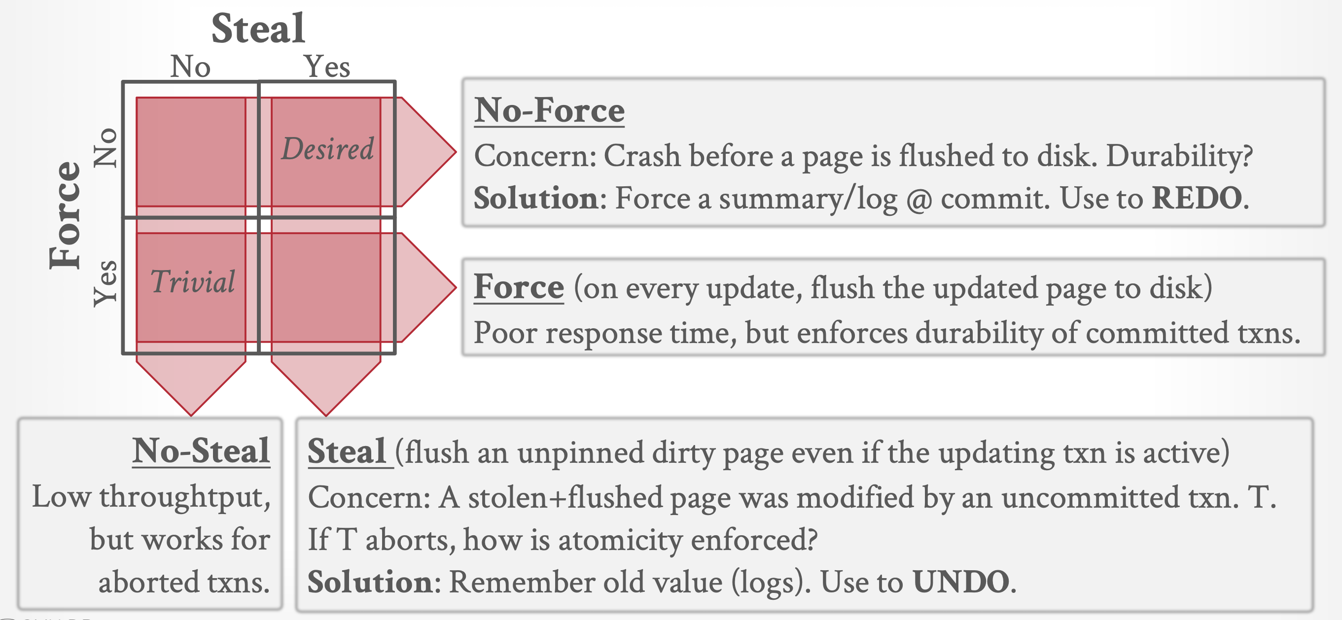
In fact, almost all DBMSs adopt the STEAL + NO-FORCE strategy.

When a block $B_1$ needs to be output to disk, all log records related to the data in $B_1$ must be written to stable storage before $B_1$ is output. The key point is that during the block output process, no write operations on that block should occur; otherwise, the write-ahead logging rule may be violated. The following special locking mechanism ensures that no write operations are in progress:

Before a transaction writes to a data item, it must acquire an exclusive lock on the block containing that data item, and release the lock immediately after the update is completed.
When outputting a block, the following sequence of operations is followed:
- Acquire an exclusive lock on the block to ensure that no transaction is writing to it.
- Output all log records associated with $B_1$ to stable storage.
- Output the block $B_1$ to disk.
- Release the lock immediately after the block output is completed.

The locks on cached blocks are unrelated to the locks used for transaction concurrency control, so releasing these locks in a non-two-phase manner does not affect transaction serializability. These short-term held locks are often referred to as latches.

During checkpoint execution, locks on cached blocks can also be used to ensure that cached blocks are not updated and that no log records are generated. This restriction can be achieved by acquiring exclusive locks on all cached blocks and the log before performing the checkpoint operation. These locks can be released immediately after the checkpoint operation is completed.

Database systems typically have a process that continuously iterates through cached blocks, writing modified cached blocks back to disk. When outputting these blocks, the aforementioned locking protocol must be followed. By continuously outputting modified blocks, the number of dirty blocks in the buffer (i.e., blocks that have been modified in the buffer but not yet written back to disk) is minimized. As a result, the number of blocks that need to be output during a checkpoint is also reduced. Additionally, when a block needs to be evicted from the buffer, it is likely that a non-dirty block is available for eviction, allowing input to proceed immediately without waiting for output to complete.

Operating System Role in Buffer Management⚓︎

The database buffer can be managed in one of the following two ways:

The database system reserves a portion of main memory as its own managed buffer (rather than being managed by the operating system).
- The drawback of this approach is that it limits the flexibility of main memory usage. The buffer must remain small enough to ensure that other applications have sufficient main memory to meet their needs. However, even when other applications are not running, the database cannot utilize all available memory. Similarly, non-database applications cannot use the portion of main memory reserved for the database buffer (even if some pages in that buffer are not currently in use).
When the database system implements its buffer within the virtual memory provided by the operating system, since the operating system is aware of the memory requirements of all processes in the system, it should theoretically decide which cache blocks must be forcibly written to disk and when. However, to ensure the requirement of write-ahead logging, the operating system should not directly write out database buffer pages but should request the database system to perform the forced output operation. At this point, the database system first writes the relevant log records to stable storage and then forcibly outputs the cache blocks to the database.
- Unfortunately, almost all contemporary operating systems have full control over virtual memory management. They reserve swap space on the disk to store virtual memory pages that are not currently in main memory. If the operating system decides to write out block $B_x$ , that block is only output to the disk’s swap space—leaving the database system unable to intervene in the output process of cache blocks.
- Therefore, if the database buffer resides in virtual memory, the data transfer between the database file and the virtual memory buffer must be managed by the database system, which enforces the write-ahead logging requirement.
- This approach may lead to additional writes to the disk. If the operating system writes out block $B_x$ , that block is not directly output to the database file but is written to the swap space of the operating system’s virtual memory. When the database system needs to write out $B_x$ , the operating system may first need to read $B_x$ from the swap space. As a result, what should have been a single output operation for $B_x$ could turn into two output operations plus an additional input operation.

Although both approaches have their flaws, we still have to choose one to implement.

15.4 Early Lock Release and Logical Undo Operations

During transaction processing, any index used can be treated as ordinary data. However, to improve concurrency, a B+ tree concurrency control algorithm can be employed to achieve early lock release in a non-two-phase manner. This idea can also be extended to recovery algorithms. The specific implementation is detailed below.

Logical Operations

Insert and delete operations are typical examples of operations that require logical rollback because they release locks early—we refer to such operations as logical operations. This early release of locks is not only crucial for indexes but also for other frequently accessed and updated system data structures. If locks are not released promptly after performing operations on such data structures, transactions will tend to execute serially, thereby affecting system performance.

Operations acquire lower-level locks during execution but release them upon completion; however, the corresponding transactions must retain high-level locks in a two-phase manner to prevent concurrent transactions from executing conflicting operations.

This early lock release allows a second insert to be performed on the same page. However, each transaction must acquire a lock on the key value to be inserted or deleted and retain it in a two-phase manner to prevent concurrent transactions from performing conflicting reads, inserts, or deletes on the same key value.

Once lower-level locks are released, an operation cannot be undone by restoring the old value of the updated data item; instead, it must be undone by executing a compensating operation—this is called a logical undo operation. The lower-level locks acquired during the operation are sufficient to perform the subsequent logical undo, for reasons explained in the next subsection.

Logical Undo Log Records

To implement logical undo operations, before executing an operation that modifies an index, the transaction creates a log record in the form of $<T_i, O_j, \text{operation-begin}>$ , where $O_j$ is the unique identifier of the operation instance. During the execution of the operation, the system generates update log records for all updates in the conventional manner. Therefore, each update caused by the operation still records the old and new values as usual.

When the operation completes, the system writes an operation-end log record in the format $<T_i, O_j, \text{operation-end}, U>$ , where $U$ represents the undo information (in simple terms: the compensating actions to be performed during the undo phase). For example, if the operation is inserting an entry into a B+ tree, the undo information $U$ must specify the deletion action to be performed, the target B+ tree, and the entry to be deleted. This method of logging operation information is called logical logging; the traditional method of recording old and new values is called physical logging, and the corresponding records are physical log records.

It should be noted that in the above scheme, logical logs are used only for undo, not for redo; redo relies entirely on physical logs. This is because after a system failure, the database state may only reflect the updates of some operations, leaving data structures such as B+ trees in an inconsistent state: neither logical redo nor logical undo can be performed. To implement logical redo/undo, it is necessary to ensure that the database state on disk is operation consistent, meaning that no partial effects of any operation should exist. However, as will be discussed later, the redo phase of the recovery scheme handles redo through physical redo, combined with rollback processing using physical log records, ensuring that the part of the database accessed by a logically undone operation reaches an operation-consistent state before execution.

If executing an operation multiple times in succession yields the same result as executing it once, we consider the operation to be idempotent. Operations such as inserting an entry into a B+ tree may not be idempotent, so the recovery algorithm must ensure that completed operations are not re-executed. In contrast, physical log records are idempotent: regardless of whether the recorded update is executed once or multiple times, the corresponding data item will retain the same value.

Transaction Rollback with Logical Undo

When rolling back transaction $T_i$ , the system scans the log records in reverse order and processes the log entries corresponding to $T_i$ as follows:

Physical log records encountered during the scan are processed according to the aforementioned rules (except for cases of skipping as explained later). Incomplete logical operations are undone using the physical log records generated by those operations.
Completed logical operations (identified by $\text{operation-end}$ records) are rolled back differently: when the system encounters a $<T_i, O_j, \text{operation-end}, U>$ log record, it performs the following special actions:
- The entire operation is rolled back using the undo information $U$ from that record. The system logs the update operations performed during the rollback as if the operation were being executed for the first time. After completing the operation rollback, the database system does not generate a $<T_i, O_j, \text{operation-end}, U>$ record; instead, it generates a $<T_i, O_j, \text{operation-abort}>$ record.
- As the reverse scan of the log continues, the system skips all log records of transaction $T_i$ until it finds $<T_i, O_j, \text{operation-begin}>$ . Once the $\text{operation-begin}$ record is located, normal processing of transaction $T_i$ log records resumes.
The system records physical undo information for update operations during rollback, rather than using only redo compensation log records. This is because a crash may occur during logical undo, and the system must complete that logical undo during recovery; to this end, restart recovery uses physical undo information to first eliminate the partial effects of the previously incomplete undo, and then re-execute the logical undo.

It should also be noted: when an operation-end log record is found during rollback, physical log records are skipped to ensure that once an operation is completed, old values from the physical log are no longer used for rollback.
If the system finds a record $<T_i, O_j, \text{operation-abort}>$ , it skips all preceding records (including the operation-end record of $O_j$ ) until it finds the $<T_i, O_j, \text{operation-begin}>$ record.
- An $operation-abort$ log record appears only when the transaction being rolled back has been partially rolled back previously. Note that logical operations may not be idempotent, so repeated execution of the same logical undo operation must be avoided. The skipping mechanism for these preceding log records ensures that, in the event of a crash during a previous rollback where the transaction was partially rolled back, the same operation is not rolled back multiple times.
When a $<T_i, \text{ abort}>$ log record is found, it indicates that the rollback of the transaction is complete. At this point, the system appends a $<T_i, \text{ abort}>$ record to the log.

15.5 ARIES

The most classic database recovery algorithm is ARIES (Algorithms for Recovery and Isolation Exploiting Semantics). It employs several new techniques to reduce recovery time and lower the overhead of checkpoint operations. Its uniqueness lies in avoiding redundant redo of already executed log operations while minimizing the amount of log records.

ARIES adopts the following techniques:

Uses log sequence numbers (LSN) to identify log records and stores LSNs in database pages to determine which operations have been applied to the pages.
Supports physiological redo operations, which physically identify the affected pages but can be logical within the page.
Implements a dirty page table mechanism to reduce unnecessary redo operations during recovery.
Employs fuzzy checkpoints, which only need to record dirty page information and related metadata without forcing dirty pages to be written out at checkpoint time. The system replaces centralized write operations during checkpoints with continuous background flushing of dirty pages.

Data Structures

Each log record in ARIES has a unique LSN. This number appears to be merely a logical identifier, but it can also be used to locate log records on disk. Typically, ARIES divides logs into multiple log files, each with its own file number. When a log file grows to a certain limit, ARIES appends subsequent log records to a new log file; the new file’s number is one higher than the previous file. Therefore, the LSN consists of the file number and the offset within that file.

Each page also maintains an identifier called PageLSN:

Whenever an update operation (whether physical or physiological) occurs on a page, the operation stores the LSN of its corresponding log record in the PageLSN field of that page.
During the redo phase of recovery, any log record with an LSN less than or equal to the page’s PageLSN value should not be applied to that page again—because the effects of those operations are already reflected on the current page.
Combined with the recording scheme that uses PageLSN as part of checkpoints (to be introduced later), ARIES can even avoid reading page data that already reflects all relevant operations on disk, thereby significantly shortening recovery time.
PageLSN is crucial for ensuring idempotency in the presence of physiological redo operations, because reapplying a physiological redo operation to a page that has already undergone it could cause erroneous changes to the page’s content.

Additionally, the DBMS records the largest log sequence number that has been flushed to disk, denoted as flushedLSN. Whenever the DBMS writes the log buffer to disk, the in-memory flushedLSN is updated accordingly.

When a page is being updated, it should not be flushed to disk, because it is impossible to reapply physiological operations based on the partially updated state of the page on disk. Therefore, ARIES uses latches on cached pages to prevent a cached page that is being updated from being written to disk. The system releases the cached page latch only after the update is complete and the relevant log record has been written to the log.

Each log record also contains the LSN of the previous log record in the same transaction, stored in the PrevLSN field. This allows all log records of a transaction to be retrieved in reverse order without reading the entire log.

In the ARIES system, special redo-only log records—compensation log records (CLRs)—are generated during transaction rollback. These serve the same purpose as the redo-only log records in the previously introduced recovery scheme. Additionally, CLRs also assume the function of operation abort log records in that scheme: they include an UndoNextLSN field, which marks the LSN of the next operation to be undone during transaction rollback. This field functions like the operation identifier of operation abort log records in the previously introduced recovery scheme, used to skip already rolled-back log records.

The DirtyPageTable (DPT) records the list of pages that have been modified in the database buffer. For each page, the table stores the PageLSN and RecLSN fields (used to identify log records that have been applied to the disk version of the page). When a page is first modified in the buffer pool and added to the DPT, the RecLSN value is set to the current end of the log; whenever a page is flushed to disk, it is removed from the DPT.

A checkpoint log record includes the DPT and the list of active transactions. For each transaction, the checkpoint log record also marks the LastLSN. A fixed location on disk also records the LSN of the most recent (complete) checkpoint log record.

The table below lists some common LSNs and their respective roles:

Name	Location	Definition
flushedLSN	Memory	The last LSN in the disk log
pageLSN	page_x	The latest update to page_x
recLSN	Dirty Page Table	The oldest update in page_x since the last flush
lastLSN	Active Transaction Table	The latest record in transaction T_i
MasterRecord	Disk	The LSN of the latest checkpoint

Recovery Algorithm

The recovery algorithm is divided into three phases:

Analysis pass: Determines which transactions need to be undone, which pages were dirty at the time of the crash, and the LSN from which the redo phase should start.
Redo pass: Starting from the LSN identified in the analysis phase, performs redo operations to replay history and restore the database to its state before the crash.
Undo pass: Rolls back all transactions that were incomplete at the time of the crash.

Analysis Pass

Preparing for the Redo Phase:

The analysis phase locates the last complete checkpoint log record and reads the DPT (Dirty Page Table) from that record.
It then sets RedoLSN to the minimum RecLSN among all pages in the DPT.
If there are no dirty pages, RedoLSN is set to the LSN of the checkpoint log record; the redo process scans the log starting from RedoLSN (all log records before this point have already been applied to the database pages on disk).
When an update operation log for a page is found, the analysis phase updates the DPT synchronously: if the page is not yet registered in the DPT, it is added, and the page’s RecLSN is set to the LSN value of the current log record.

Preparing for the Undo Phase:

Initialize the undo list with the transaction list from the checkpoint log record, and read the LSN of the last log record for each transaction in the undo list from the checkpoint record. Then scan forward from the checkpoint:
- Whenever a log record belonging to a transaction not in the undo list is found, that transaction is added to the undo list;
- When a log record indicating the end of a transaction (commit, not abort) is encountered, that transaction is removed from the undo list.
All transactions remaining in the undo list must be rolled back during the subsequent undo process.
The analysis phase also tracks the last record of each transaction in the undo list for use in the undo phase.

This phase does not read the contents of the memory buffer.

Redo Pass

The redo phase replays history by redoing all operations that have not yet been reflected on the disk pages. This phase scans the log forward starting from RedoLSN. Whenever an update log record is found, the following operations are performed:

If the target page is not in the DPT, or the LSN of the update log record is less than the RecLSN value of the corresponding page in the DPT, this log record is skipped;
Otherwise, the redo phase reads the page from disk. If its PageLSN is less than the LSN of the current log record, the log record is re-executed.

Note: As long as either condition is not met, it means that the modification effect of the log record has already been reflected on the page; conversely, it indicates that the modification effect has not yet been reflected on the page. Since ARIES allows non-idempotent physiological log records, if the modification of a log record has already been applied to the page, it should not be redone again. When the first condition is not met, there is no need to even fetch the page from disk to check its PageLSN value.

Undo Pass

During the undo phase, a reverse scan of the log is performed to roll back all transactions in the undo list. This phase only checks the log records of transactions in the undo list; the last LSN recorded in the analysis phase is used to locate the final log record of each transaction to be undone.

Whenever an update log record is found, whether it is a rollback of a transaction during normal processing or an undo operation during restart recovery, the undo action is executed based on that record. The undo phase generates a CLR containing the executed (which must be physiological) undo operation, and sets the UndoNextLSN value of this CLR to the PrevLSN value of the original update log record.

If a CLR is encountered, its UndoNextLSN field indicates the LSN of the next log record to be undone for that transaction—meaning that the subsequent log records of that transaction have already been rolled back.
For other log records that are not CLRs, the next record to be undone is determined by their PrevLSN field.

When processing resumes after each interruption, the system selects the largest “next LSN to process” among all transactions in the undo list as the target for the next operation.

Finally, all undone transactions must be aborted, so CLRs related to the abort need to be inserted (e.g., $<T_i\ \text{abort}>$ ).

Other Features

Nested Top Actions: ARIES allows recording operations that should not be undone even if the transaction is rolled back. For example, if a transaction allocates a page for a relation, the page allocation should not be undone even if the transaction is rolled back, because other transactions may have already stored records on that page. Such operations that should not be undone are called nested top actions.
- These operations can be modeled as operations with an empty undo action.
- In ARIES, such operations are implemented by creating a virtual CLR, whose UndoNextLSN is set so that when the transaction is rolled back, the log records generated by this operation are skipped.
Recovery Independence: Certain pages can be recovered independently of other pages, allowing them to remain usable even while other pages are being recovered. If some pages on disk fail, they can be recovered individually without interrupting transaction processing on other pages.
Savepoints: Transactions can record savepoints and can partially roll back to a specific savepoint.
- This is particularly useful for deadlock handling, as a transaction can roll back to a point where it can release the required locks and then restart from that point.
- Programmers can also use savepoints to partially undo a transaction and then continue execution; this approach is suitable for handling certain types of errors detected during transaction execution.
Fine-Grained Locking: The ARIES recovery algorithm can work with index concurrency control algorithms that allow tuple-level locking instead of page-level locking on indexes, significantly improving concurrency performance.
Recovery Optimizations:
- The DPT can be used to prefetch pages during the redo phase.
- Out-of-order redo can also be supported: for pages being read from disk, redo operations can be deferred until the page is loaded; meanwhile, the system can continue processing other log records.

About this Post

This post is written by Rinic, licensed under CC BY-NC 4.0.